Alpha–beta pruning facts for kids

Quick facts for kids
Alpha–beta pruning

Class	Search algorithm
Worst-case performance
Best-case performance

Alpha–beta pruning is a search algorithm that seeks to decrease the number of nodes that are evaluated by the minimax algorithm in its search tree. It is an adversarial search algorithm used commonly for machine playing of two-player games (Tic-tac-toe, Chess, Connect 4, etc.). It stops evaluating a move when at least one possibility has been found that proves the move to be worse than a previously examined move. Such moves need not be evaluated further. When applied to a standard minimax tree, it returns the same move as minimax would, but prunes away branches that cannot possibly influence the final decision.

History

Allen Newell and Herbert A. Simon who used what John McCarthy calls an "approximation" in 1958 wrote that alpha–beta "appears to have been reinvented a number of times". Arthur Samuel had an early version for a checkers simulation. Richards, Timothy Hart, Michael Levin and/or Daniel Edwards also invented alpha–beta independently in the United States. McCarthy proposed similar ideas during the Dartmouth workshop in 1956 and suggested it to a group of his students including Alan Kotok at MIT in 1961. Alexander Brudno independently conceived the alpha–beta algorithm, publishing his results in 1963. Donald Knuth and Ronald W. Moore refined the algorithm in 1975. Judea Pearl proved its optimality in terms of the expected running time for trees with randomly assigned leaf values in two papers. The optimality of the randomized version of alpha–beta was shown by Michael Saks and Avi Wigderson in 1986.

Core idea

A game tree can represent many two-player zero-sum games, such as chess, checkers, and reversi. Each node in the tree represents a possible situation in the game. Each terminal node (outcome) of a branch is assigned a numeric score that determines the value of the outcome to the player with the next move.

The algorithm maintains two values, alpha and beta, which respectively represent the minimum score that the maximizing player is assured of and the maximum score that the minimizing player is assured of. Initially, alpha is negative infinity and beta is positive infinity, i.e. both players start with their worst possible score. Whenever the maximum score that the minimizing player (i.e. the "beta" player) is assured of becomes less than the minimum score that the maximizing player (i.e., the "alpha" player) is assured of (i.e. beta < alpha), the maximizing player need not consider further descendants of this node, as they will never be reached in the actual play.

To illustrate this with a real-life example, suppose somebody is playing chess, and it is their turn. Move "A" will improve the player's position. The player continues to look for moves to make sure a better one hasn't been missed. Move "B" is also a good move, but the player then realizes that it will allow the opponent to force checkmate in two moves. Thus, other outcomes from playing move B no longer need to be considered since the opponent can force a win. The maximum score that the opponent could force after move "B" is negative infinity: a loss for the player. This is less than the minimum position that was previously found; move "A" does not result in a forced loss in two moves.

Improvements over naive minimax

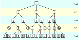
An illustration of alpha–beta pruning. The grayed-out subtrees don't need to be explored (when moves are evaluated from left to right), since it is known that the group of subtrees as a whole yields the value of an equivalent subtree or worse, and as such cannot influence the final result. The max and min levels represent the turn of the player and the adversary, respectively.

The benefit of alpha–beta pruning lies in the fact that branches of the search tree can be eliminated. This way, the search time can be limited to the 'more promising' subtree, and a deeper search can be performed in the same time. Like its predecessor, it belongs to the branch and bound class of algorithms. The optimization reduces the effective depth to slightly more than half that of simple minimax if the nodes are evaluated in an optimal or near optimal order (best choice for side on move ordered first at each node).

With an (average or constant) branching factor of b, and a search depth of d plies, the maximum number of leaf node positions evaluated (when the move ordering is pessimal) is O(b×b×...×b) = O(b^d) – the same as a simple minimax search. If the move ordering for the search is optimal (meaning the best moves are always searched first), the number of leaf node positions evaluated is about O(b×1×b×1×...×b) for odd depth and O(b×1×b×1×...×1) for even depth, or . In the latter case, where the ply of a search is even, the effective branching factor is reduced to its square root, or, equivalently, the search can go twice as deep with the same amount of computation. The explanation of b×1×b×1×... is that all the first player's moves must be studied to find the best one, but for each, only the second player's best move is needed to refute all but the first (and best) first player move—alpha–beta ensures no other second player moves need be considered. When nodes are considered in a random order (i.e., the algorithm randomizes), asymptotically, the expected number of nodes evaluated in uniform trees with binary leaf-values is . For the same trees, when the values are assigned to the leaf values independently of each other and say zero and one are both equally probable, the expected number of nodes evaluated is , which is much smaller than the work done by the randomized algorithm, mentioned above, and is again optimal for such random trees. When the leaf values are chosen independently of each other but from the interval uniformly at random, the expected number of nodes evaluated increases to in the limit, which is again optimal for these kind random trees. Note that the actual work for "small" values of is better approximated using .

A chess program that searches four plies with an average of 36 branches per node evaluates more than one million terminal nodes. An optimal alpha-beta prune would eliminate all but about 2,000 terminal nodes, a reduction of 99.8%.

An animated pedagogical example that attempts to be human-friendly by substituting initial infinite (or arbitrarily large) values for emptiness and by avoiding using the negamax coding simplifications.

Normally during alpha–beta, the subtrees are temporarily dominated by either a first player advantage (when many first player moves are good, and at each search depth the first move checked by the first player is adequate, but all second player responses are required to try to find a refutation), or vice versa. This advantage can switch sides many times during the search if the move ordering is incorrect, each time leading to inefficiency. As the number of positions searched decreases exponentially each move nearer the current position, it is worth spending considerable effort on sorting early moves. An improved sort at any depth will exponentially reduce the total number of positions searched, but sorting all positions at depths near the root node is relatively cheap as there are so few of them. In practice, the move ordering is often determined by the results of earlier, smaller searches, such as through iterative deepening.

Additionally, this algorithm can be trivially modified to return an entire principal variation in addition to the score. Some more aggressive algorithms such as MTD(f) do not easily permit such a modification.

Pseudocode

The pseudo-code for depth limited minimax with alpha–beta pruning is as follows:

Implementations of alpha–beta pruning can often be delineated by whether they are "fail-soft," or "fail-hard". With fail-soft alpha–beta, the alphabeta function may return values (v) that exceed (v < α or v > β) the α and β bounds set by its function call arguments. In comparison, fail-hard alpha–beta limits its function return value into the inclusive range of α and β. The main difference between fail-soft and fail-hard implementations is whether α and β are updated before or after the cutoff check. If they are updated before the check, then they can exceed initial bounds and the algorithm is fail-soft.

The following pseudo-code illustrates the fail-hard variation.

function alphabeta(node, depth, α, β, maximizingPlayer) is if depth == 0 or node is terminal then return the heuristic value of node if maximizingPlayer then value := −∞ for each child of node do value := max(value, alphabeta(child, depth − 1, α, β, FALSE)) if value > β then break (* β cutoff *) α := max(α, value) return value else value := +∞ for each child of node do value := min(value, alphabeta(child, depth − 1, α, β, TRUE)) if value < α then break (* α cutoff *) β := min(β, value) return value

(* Initial call *) alphabeta(origin, depth, −∞, +∞, TRUE)

The following pseudocode illustrates fail-soft alpha-beta.

function alphabeta(node, depth, α, β, maximizingPlayer) is if depth == 0 or node is terminal then return the heuristic value of node if maximizingPlayer then value := −∞ for each child of node do value := max(value, alphabeta(child, depth − 1, α, β, FALSE)) α := max(α, value) if value ≥ β then break (* β cutoff *) return value else value := +∞ for each child of node do value := min(value, alphabeta(child, depth − 1, α, β, TRUE)) β := min(β, value) if value ≤ α then break (* α cutoff *) return value

(* Initial call *) alphabeta(origin, depth, −∞, +∞, TRUE)

Heuristic improvements

Further improvement can be achieved without sacrificing accuracy by using ordering heuristics to search earlier parts of the tree that are likely to force alpha–beta cutoffs. For example, in chess, moves that capture pieces may be examined before moves that do not, and moves that have scored highly in earlier passes through the game-tree analysis may be evaluated before others. Another common, and very cheap, heuristic is the killer heuristic, where the last move that caused a beta-cutoff at the same tree level in the tree search is always examined first. This idea can also be generalized into a set of refutation tables.

Alpha–beta search can be made even faster by considering only a narrow search window (generally determined by guesswork based on experience). This is known as aspiration search. In the extreme case, the search is performed with alpha and beta equal; a technique known as zero-window search, null-window search, or scout search. This is particularly useful for win/loss searches near the end of a game where the extra depth gained from the narrow window and a simple win/loss evaluation function may lead to a conclusive result. If an aspiration search fails, it is straightforward to detect whether it failed high (high edge of window was too low) or low (lower edge of window was too high). This gives information about what window values might be useful in a re-search of the position.

Over time, other improvements have been suggested, and indeed the Falphabeta (fail-soft alpha–beta) idea of John Fishburn is nearly universal and is already incorporated above in a slightly modified form. Fishburn also suggested a combination of the killer heuristic and zero-window search under the name Lalphabeta ("last move with minimal window alpha–beta search").

Other algorithms

Since the minimax algorithm and its variants are inherently depth-first, a strategy such as iterative deepening is usually used in conjunction with alpha–beta so that a reasonably good move can be returned even if the algorithm is interrupted before it has finished execution. Another advantage of using iterative deepening is that searches at shallower depths give move-ordering hints, as well as shallow alpha and beta estimates, that both can help produce cutoffs for higher depth searches much earlier than would otherwise be possible.

Algorithms like SSS*, on the other hand, use the best-first strategy. This can potentially make them more time-efficient, but typically at a heavy cost in space-efficiency.

See also

In Spanish: Poda alfa-beta para niños