Lotka–Volterra equations facts for kids

The Lotka–Volterra equations are also known as the Lotka–Volterra predator–prey model. They are a set of two special math equations. These equations help us understand how two different groups of animals (or species) interact. One group is the predator (like a fox), and the other is the prey (like a rabbit).

These equations show how the numbers of predators and prey change over time. They help scientists study how these groups affect each other in nature.

The equations look like this: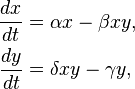

Here's what the letters mean:

• The letter x stands for the number of prey animals. For example, it could be the number of rabbits in an area.
• The letter y stands for the number of predator animals. For example, it could be the number of foxes in the same area.
• and show how fast the numbers of prey and predators are growing or shrinking.
• t means time.
• The letters α, β, γ, and δ are special numbers. They describe things like how fast prey grow or how many predators die. All these numbers are positive.

The Lotka–Volterra model helps us see how populations change. It shows that these changes happen smoothly and continuously.

What the Model Shows About Nature

This graph shows the numbers of snowshoe hare (yellow) and Canada lynx (black) furs sold. Canada lynxes eat snowshoe hares.

Even though the model is simple, it teaches us two important things about predator and prey populations:

First, the numbers of predators and prey often go up and down in a cycle. We can see this in real life. For example, the numbers of lynx and snowshoe hare furs sold by the Hudson's Bay Company show these ups and downs. The same patterns are seen with moose and wolf populations in Isle Royale National Park.

Second, the model shows that if prey animals have a better environment (like more food), it helps the predators more than the prey. For example, during World War I, less fishing meant more prey fish. This led to more predatory fish being caught, not more prey fish. This idea is sometimes called the "paradox of the pesticides."

Another example is when scientists added iron to the ocean. Iron helps tiny ocean plants (phytoplankton) grow. Scientists hoped this would help remove carbon dioxide from the air. But the phytoplankton were quickly eaten by other tiny animals (zooplankton) and small fish. This mostly led to more predators, not more phytoplankton. This matches what the Lotka–Volterra model predicts.

History of the Model

The Lotka–Volterra model was first thought of by Alfred J. Lotka in 1910. He used it to explain how chemicals react. In 1920, he used the equations to study how plants and plant-eating animals interact. Then, in 1925, he wrote a book about it.

At the same time, in 1926, a mathematician named Vito Volterra also published the same equations. Volterra became interested in this idea because of a marine biologist named Umberto D'Ancona. D'Ancona was studying fish catches in the Adriatic Sea. He noticed that during World War I (1914–18), fewer people were fishing. But the percentage of predatory fish caught actually went up! This seemed strange.

Volterra used his math skills to create a model that could explain D'Ancona's observation. He did this without knowing about Lotka's work at first. Later, he gave credit to Lotka, and that's why the model is known as the "Lotka-Volterra model."

Scientists have since made the model more complex. They have added more details to better explain how predators and prey interact in nature.

How the Equations Work

The Lotka–Volterra equations show that the numbers of predators and prey go up and down in a regular pattern. These patterns repeat over time.

Imagine a graph where one line shows the number of rabbits and another shows the number of foxes. If you start with 10 rabbits and 10 foxes, the graph would show how their numbers change. The rabbits might increase first, then the foxes, then the rabbits decrease, and so on.

Population changes for rabbits and foxes over time.

This graph shows how the numbers of predators and prey relate to each other.

You can also plot these numbers on a special graph called a "phase-space plot." This graph doesn't show time directly. Instead, one side shows the number of prey, and the other side shows the number of predators. The lines on this graph form closed loops. This means the populations keep cycling through the same patterns.

One challenge with this simple model is that sometimes it predicts very, very small numbers of animals. For example, it might predict a tiny fraction of a rabbit. In real life, if the number of rabbits gets too low, they might all die out. Then, the foxes would also die out because they have no food. This is a limit of the simple model.

How the System Changes

In this model, predators do well when there are many prey animals. But then, they eat too much prey, and their own numbers start to drop. When there are fewer predators, the prey population can grow again. This creates a repeating cycle of growth and decline for both groups.

When Populations Are Balanced

A population is balanced when the numbers of both species are not changing. This happens when the growth rates for both prey and predators are zero.

The equations show two main situations where this balance happens: 1. When both species are extinct (their numbers are zero). If there are no animals, their numbers will stay at zero. 2. When both species have a steady, non-zero number. This is a "fixed point" where their populations stay the same over time. The exact numbers depend on the special values (α, β, γ, δ) we talked about earlier.

How Stable Are the Balance Points?

Scientists use math to figure out if these balance points are stable.

Extinction Point

The point where both species are extinct (0 prey, 0 predators) is not stable. This means if you start with even a tiny number of animals, they won't stay at zero. The populations will grow or change. So, in this model, it's hard for both species to go extinct unless one is completely wiped out first.

Oscillation Point

The second balance point, where both populations have steady, non-zero numbers, is stable. But it's a special kind of stable point. It means the populations don't just stay still. Instead, they cycle around this point. The numbers of predators and prey go up and down in a regular, repeating pattern, like waves. This is why we see the populations oscillating in the graphs.

The speed of these cycles depends on the special numbers (α and γ) in the equations.

See also

In Spanish: Ecuaciones de Lotka-Volterra para niños

Images for kids

• 

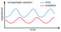
  This image shows the cycles of predator and prey populations over time.

• 

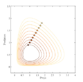
  This graph shows how predator and prey numbers relate to each other in a cycle.