Pearson correlation coefficient facts for kids

In statistics, the Pearson correlation coefficient (also called Pearson's r) is a special number. It helps us understand how strongly two sets of data are connected. It tells us if they move together in a straight line.

Imagine you have two lists of numbers, like the height of students and their shoe sizes. The Pearson correlation coefficient tells you if taller students tend to have bigger shoe sizes.

This number is always between -1 and 1.

• If it's close to 1, it means the two things go up or down together very strongly. Like, if you study more, your grades usually go up.
• If it's close to -1, it means one thing goes up while the other goes down. Like, the more you exercise, the less time you might spend watching TV.
• If it's close to 0, it means there's no clear straight-line connection between the two things. Like, the number of pets you have and your favorite color probably have no connection.

For example, if you look at the age and height of teenagers, you'd expect a Pearson correlation coefficient greater than 0 but less than 1. This means as teenagers get older, they usually get taller, but it's not a perfect match for everyone.

Examples of how different correlation numbers look on a graph.

More examples of how points on a graph show different correlation numbers.

Who created it?

This idea was first introduced by Francis Galton in the 1880s. Later, Karl Pearson developed it further. The math formula for it was actually published by Auguste Bravais even earlier, in 1844.

What does it mean?

The Pearson correlation coefficient measures how much two things change together. It looks at how much they vary from their average values. It's like seeing if two friends tend to walk at the same speed or if one always walks faster.

For a whole group

When we talk about a whole group of people or things (like all teenagers in a country), we use the Greek letter ρ (pronounced "rho") for the Pearson correlation coefficient.

It compares how much two things, let's say X (like height) and Y (like weight), change together. It divides this shared change by how much each thing changes on its own. This makes sure the final number is always between -1 and 1.

For a small group (sample)

When we only look at a small part of a group (like 50 teenagers from one school), we call it a "sample." For a sample, we use the letter r for the Pearson correlation coefficient.

To find r, we collect data pairs, like (height, weight) for each teenager. Then, we use a formula that compares each person's height to the average height and their weight to the average weight.

The formula looks complicated, but computers and calculators can do it easily for us: 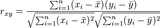Here:

• n is the number of people in your small group.
• x_i and y_i are the individual measurements for each person.
• is the average height, and is the average weight.

Important facts about it

The Pearson correlation coefficient always falls between -1 and 1.

• If it's exactly 1 or -1, it means all the data points line up perfectly on a straight line.
• It doesn't matter if you swap the two things around; the correlation between X and Y is the same as between Y and X.
• The correlation number doesn't change if you add a constant number to all your data points or multiply them by a positive number. For example, if you measure height in inches instead of centimeters, the correlation with weight won't change.

How to use it to make guesses

Scientists often use the Pearson correlation coefficient to test ideas or make predictions.

One common goal is to see if there's a real connection (correlation) between two things, or if it's just by chance. For example, is there a real correlation between hours spent playing video games and test scores, or is any connection just random?

Another goal is to figure out a range where the true correlation likely falls. This range is called a confidence interval.

Using a shuffle test

A "permutation test" is like a shuffle test. 1. You take your original pairs of data (like height and weight). 2. Then, you randomly mix up one set of data. For example, you keep the heights in order but randomly shuffle the weights. 3. You calculate the correlation for this new, shuffled data. 4. You repeat steps 2 and 3 many, many times. 5. Finally, you see how many of these shuffled correlations are stronger than your original correlation. If very few are stronger, it means your original correlation is probably real and not just due to chance.

Using a "bootstrap" method

The "bootstrap" method is another way to guess the true correlation. 1. You take your original data pairs. 2. You create new sets of data by picking pairs from your original set, but you can pick the same pair more than once. 3. You calculate the correlation for each new set. 4. After doing this many times, you look at all the correlations you got. This helps you estimate the range where the true correlation likely is.

Critical values of Pearson's correlation coefficient. This graph helps you see how strong a correlation needs to be to be considered "real" based on how many data points you have.

How good is the data?

The Pearson correlation coefficient works best when your data is spread out in a certain way, like a bell curve.

How many data points do you need?

• If you have a lot of data points and they follow a "normal" pattern, the sample correlation coefficient is a very good guess of the true correlation.
• If you have a lot of data points but they don't follow a "normal" pattern, the sample correlation is still a good guess, but maybe not the best possible.
• If you have only a few data points, the sample correlation might not be a perfect guess.

What if there are weird data points?

Sometimes, you might have "outliers" – data points that are very different from the rest. For example, if you're measuring the height of 12-year-olds and one person is an adult, that's an outlier. Outliers can make the Pearson correlation coefficient misleading.

It's always a good idea to look at a scatterplot (a graph with dots for each data point) to see if there are any outliers or if the data doesn't look like a straight line. If it doesn't, other ways of measuring connections might be better.

Other types of correlation

There are other ways to measure how things are connected, depending on what you're studying.

Weighted correlation

Sometimes, some data points are more important than others. A "weighted" correlation lets you give more importance to certain data points when calculating the connection.

Pearson's distance

You can also use the Pearson correlation coefficient to measure the "distance" between two things. If they are strongly correlated (close to 1), their distance is small. If they are not correlated (close to 0), their distance is larger. If they are negatively correlated (close to -1), their distance is the largest.

Circular correlation

If your data involves directions or angles (like wind direction), you can use a "circular correlation coefficient." This is a special version of Pearson's correlation designed for data that goes in a circle.

Partial correlation

Imagine you want to see the connection between ice cream sales and drowning incidents. You might find a strong positive correlation. But is it because ice cream causes drowning? Probably not! It's likely because both increase in hot weather. "Partial correlation" helps you look at the connection between two things while removing the influence of a third thing (like temperature).

Making variables uncorrelated

It's possible to change a set of data so that all the variables in it no longer have any straight-line correlation with each other. This is like taking a group of friends who always walk together and making them all walk in their own directions. This process is used in advanced data analysis.

Computer programs that calculate it

Many computer programs and tools can calculate the Pearson correlation coefficient for you:

• R: A programming language for statistics, it uses `cor(x, y)` or `cor.test(x, y)`.
• Python: A popular programming language, its SciPy library has `pearsonr(x, y)`.
• Excel: The spreadsheet program has a function called `correl(array1, array2)`.

In Spanish: Coeficiente de correlación de Pearson para niños

Images for kids

• 

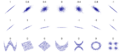
  Examples of scatter diagrams with different values of correlation coefficient (ρ)

• 

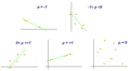
  Several sets of (x, y) points, with the correlation coefficient of x and y for each set. The correlation reflects the strength and direction of a linear relationship (top row), but not the slope of that relationship (middle), nor many aspects of nonlinear relationships (bottom). N.B.: the figure in the center has a slope of 0 but in that case the correlation coefficient is undefined because the variance of Y is zero.

• 

  Critical values of Pearson's correlation coefficient that must be exceeded to be considered significantly nonzero at the 0.05 level.