Predator-prey equations facts for kids

The predator-prey equations are a set of two special math formulas. They help us understand how two groups of animals depend on each other. One group is the prey, which is food for the other group, the predator. Both prey and predator groups can grow if conditions are right.
A scientist named Alfred J. Lotka first found these equations in 1925. Another scientist, Vito Volterra, found them on his own in 1926. Because of this, the equations are also called the Lotka-Volterra equations.
These equations are a type of differential equation. This means they describe how things change over time.
Contents
How the Equations Work
The predator-prey equations work best when certain things are true:
- The prey animals always find enough food to eat.
- The number of predators depends only on how many prey animals there are.
- How fast a group grows or shrinks depends on its current size.
- The environment stays the same and doesn't favor one animal over the other.
- Predators can eat as much as they need.
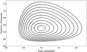
When these conditions are met, the equations show a clear pattern. They predict that the numbers of predators and prey will keep changing in a steady, repeating way. This means that new generations of both animals are always appearing.
Lotka-Volterra Rules
The solutions to these equations lead to three main rules, often called the Lotka-Volterra rules:
- The numbers of predators and prey change in cycles. The predator numbers go up and down after the prey numbers do.
- Over long periods, the average number of predators and prey stays about the same. This is true as long as the environment doesn't change.
- If the number of predators goes down, the number of prey animals will usually go up.
Real-World Examples
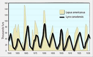
Scientists have used these equations to understand real animal populations. For example, the numbers of snowshoe hares and Canada lynx in Canada show these cycles. Lynxes eat hares, so their numbers follow the hare population.
Vito Volterra also looked at fish caught in the Mediterranean Sea. He studied numbers of sharks and other fish they eat. He noticed something interesting between 1915 and 1920. During the First World War, less fishing happened. This meant there were more prey fish. Because of this, the number of sharks (predators) increased. After the war, fishing went back to normal. This reduced the prey fish, which then led to fewer sharks.
Here are some of the numbers Volterra looked at, showing the percentage of sharks caught:
| 1905 | 1910 | 1911 | 1912 | 1913 | 1914 | 1915 | 1916 | 1917 | 1918 | 1919 | 1920 | 1921 | 1922 | 1923 | |
| Trieste | – | 5.7 | 8.8 | 9.5 | 15.7 | 14.6 | 7.6 | 16.2 | 15.4 | – | 19.9 | 15.8 | 13.3 | 10.7 | 10.2 |
| Fiume | – | – | – | – | - | 11.9 | 21.4 | 22.1 | 21.2 | 36.4 | 27.3 | 16.0 | 15.9 | 14.8 | 10.7 |
| Venice | 21.8 | – | – | – | - | – | – | - | – | – | 30.9 | 25.3 | 25.9 | 26.8 | 26.6 |
Expanding the Model
The predator-prey equations have been used as a starting point for other studies. Volterra himself made them more complex. He wanted to include intraspecific competition. This happens when animals of the same species compete for limited food or space. Intraspecific competition is important because it helps control how many animals can live in an area. It also helps animals adapt to changes in their environment over time.
Most of Volterra's later work focused on making the model work for more than two types of animals interacting.
See also
 In Spanish: Ecuaciones de Lotka-Volterra para niños


