Neural network (machine learning) facts for kids

An artificial neural network is an interconnected group of nodes, like tiny brain cells. Each circle is a small "artificial neuron," and the arrows show how they connect and send signals to each other.

In machine learning, a neural network (also called an artificial neural network or neural net) is a special computer program. It's designed to work a bit like a real brain. These networks are inspired by how biological neural networks in animals think and learn.

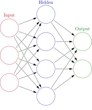
A neural network is made of many connected parts called artificial neurons. These are like the neurons in your brain. They are linked together by "edges," which are like the synapses in your brain. Each artificial neuron gets signals from others. It then processes these signals and sends new ones to other connected neurons.

The "signal" is a number. Each neuron figures out its output using a special math rule. This rule is called an activation function. The strength of each connection is set by a "weight." These weights change as the network learns new things.

Usually, neurons are grouped into layers. Each layer does a different job with the information it gets. Signals start at the first layer, called the input layer. They then travel through other layers, known as hidden layers. Finally, they reach the output layer. If a network has at least two hidden layers, it's often called a deep neural network.

Artificial neural networks are used for many tasks. They can help with predictive modeling, controlling things, and solving problems in artificial intelligence. They learn from experience. They can also find patterns and make sense of lots of information that might seem unrelated.

How Neural Networks Learn

Neural networks learn by trying to get things right. This process is called "training." Imagine you are teaching a computer to tell the difference between cats and dogs. You would show it many pictures of cats and dogs. For each picture, you would tell the computer if it's a cat or a dog.

The network tries to guess what's in the picture. If it guesses wrong, it adjusts its internal settings. These settings are the "weights" we talked about earlier. It keeps adjusting them until its guesses are very close to the correct answers. This is like practicing until you get something perfect.

This learning often uses a method called backpropagation. It helps the network figure out how much each connection's weight needs to change. This way, the network gets better at understanding new information it hasn't seen before.

A simple example of training a neural network. The network learns to spot starfish and sea urchins from many pictures. It connects features like "ringed texture" to starfish.

After training, the network can find a starfish in a new picture. Sometimes, it might get a weak signal for something else, like a sea urchin, if a feature is similar. This could lead to a small mistake.

The Story of Neural Networks

Neural networks have a long and interesting history. Their ideas go back over 200 years!

Early Ideas and Simple Networks

The very first ideas for these networks came from statistics. A simple type of network is like a basic math equation. It takes inputs, multiplies them by weights, and adds them up. This method was used by mathematicians like Adrien-Marie Legendre and Gauss in the early 1800s. They used it to predict things like how planets move.

Later, in the 1940s, scientists started thinking about how real brains work. Warren McCulloch and Walter Pitts (1943) created a simple model of a neuron. This led to two paths: one focused on biology, and the other on using these ideas for artificial intelligence.

In the late 1940s, Donald O. Hebb suggested a way neurons might learn. This idea, called Hebbian learning, was used in many early networks. Scientists like Farley and Wesley A. Clark (1954) even built machines to try out these ideas.

The Perceptron and Early Excitement

In 1958, a psychologist named Frank Rosenblatt created the "perceptron." This was one of the first working artificial neural networks. It caused a lot of excitement! People thought these networks could soon think like humans. This led to a "Golden Age of AI" with lots of funding.

However, these early perceptrons were simple. They couldn't solve more complex problems, like the "exclusive-or" puzzle. This problem involves telling apart patterns that are not simply "on" or "off." This led to a slowdown in research in the US.

Deep Learning Begins

Even though research slowed, some important work continued. In 1965, Alexey Ivakhnenko in Ukraine developed the "Group method of data handling." This was the first working "deep learning" algorithm. It could train networks with many layers. In 1967, Shun'ichi Amari published the first deep network trained with a method called stochastic gradient descent.

In 1969, Kunihiko Fukushima introduced a key part of modern networks: the ReLU activation function. This function helps neurons decide when to send a signal. It's now very popular in deep learning.

Backpropagation and Smarter Learning

A big breakthrough was backpropagation. This is a clever way for networks to learn from their mistakes. It was first described in its modern form by Seppo Linnainmaa in 1970. Later, Paul Werbos applied it to neural networks in 1982. David E. Rumelhart and others helped make it widely known in 1986. Backpropagation lets networks adjust their weights much more efficiently.

Seeing with Convolutional Networks

In 1979, Kunihiko Fukushima created the Neocognitron. This was the start of convolutional neural networks (CNNs). CNNs are very good at understanding images. They use special layers to find patterns like edges and shapes.

In 1989, Yann LeCun and his team created a famous CNN called LeNet. It was used by banks to read handwritten ZIP codes on mail. This showed how powerful CNNs could be for tasks like recognizing handwriting.

Networks with Memory: Recurrent Networks

Scientists also developed recurrent neural networks (RNNs). These networks have "memory." They can use information from past steps to help with current tasks. This is useful for things like understanding speech or predicting what comes next in a sequence.

Early RNNs, like the Jordan network (1986) and Elman network (1990), helped study how our minds work. However, training deep RNNs was hard.

In 1991, Jürgen Schmidhuber proposed ideas like "neural history compressor" to help RNNs learn over longer periods. In 1993, his system solved a "Very Deep Learning" task. It needed over 1000 layers of memory!

In 1991, Sepp Hochreiter found a problem called the "vanishing gradient problem." This made it hard for deep RNNs to learn. He and Schmidhuber then created long short-term memory (LSTM) networks. LSTMs are much better at remembering things over a long time. They became the standard for RNNs.

The Rise of Modern Deep Learning

Between 2009 and 2012, neural networks started winning major competitions. They began to perform as well as, or even better than, humans at tasks like image recognition.

In 2012, a CNN called AlexNet won the huge ImageNet competition. This was a big moment! It showed that deep learning could solve very complex problems. Soon after, Andrew Ng and Jeff Dean created a network that learned to recognize things like cats just by watching unlabeled videos. This showed the power of "unsupervised learning."

More powerful computers, especially GPUs (graphics processing units), helped these networks grow much larger. This led to the "deep learning" boom we see today.

In 2014, Ian Goodfellow and others created Generative adversarial networks (GANs). GANs are two networks that compete. One creates new images, and the other tries to tell if they are real or fake. This led to amazing results, like realistic fake images and videos (called deepfakes).

Later, Diffusion models (2015) became even better at creating images. Systems like DALL·E 2 and Stable Diffusion can now create stunning images from simple text descriptions.

In 2015, two new techniques, the highway network and the residual neural network (ResNet), helped train even "very deep" networks with 20 to 30 layers or more. These methods solved the "degradation" problem, where adding too many layers made networks worse.

The Transformer Era

Around 2017, a new type of network called the "Transformer" was developed. This architecture is very good at understanding language. It uses something called "attention mechanisms" to focus on important parts of text.

Transformers have become the top choice for natural language processing. Many modern large language models like ChatGPT, GPT-4, and BERT use this powerful design. They help us with tasks like writing, translating, and answering questions.

Images for kids

• 

  Neuron and myelinated axon, with signal flow from inputs at dendrites to outputs at axon terminals

• 

  Confidence analysis of a neural network

See also