
Logistic regression facts for kids
The logistic model (or logit model) is a way to predict the chance of something happening. Imagine you want to know if a student will pass an exam. Logistic regression helps figure out the probability (how likely it is) of that event (passing) based on things like how many hours they studied.
In statistics, this model helps us understand how different factors (like study hours) affect the chance of a "yes" or "no" outcome. For example, it can predict if a patient will get better, or if a customer will buy a product. It's like a special kind of regression analysis used when the answer isn't a number (like a grade from 0-100), but a choice between two things (like pass or fail).

Since the 1970s, the logistic model has been very popular for predicting these "yes/no" situations. It can also be used for more than two choices, like predicting if an image shows a cat, dog, or lion.
The math behind it helps turn the "log-odds" (a way to measure likelihood) into a simple probability between 0 (no chance) and 1 (certain chance). This special function is called the logistic function, which is where the name comes from!
Contents
- What is Logistic Regression Used For?
- A Simple Example: Passing an Exam
- How Logistic Regression Works
- Finding the Best Model
- Checking How Good the Model Is
- Why Logistic Regression is Different from Linear Regression
- History of Logistic Regression
- More Advanced Types of Logistic Regression
- Software for Logistic Regression
- Images for kids
- See also
What is Logistic Regression Used For?
Logistic regression is used in many different areas. It helps people make predictions in machine learning, medicine, and social studies.
- In Medicine: Doctors use it to predict if a patient might get a certain disease, like diabetes or heart disease. They look at things like age, gender, body mass index, and blood test results. It can also help predict how likely an injured patient is to survive.
- In Social Sciences: Researchers might use it to predict how a person will vote in an election, based on their age, income, or where they live.
- In Engineering: Engineers can use it to predict the chance of a machine part failing.
- In Marketing: Companies use it to guess if a customer will buy a product or stop using a service.
- In Economics: It can predict if someone will join the workforce or if a homeowner might struggle to pay their mortgage.
A Simple Example: Passing an Exam
Let's look at a simple example to see how logistic regression works.
The Problem
Imagine we have 20 students. They each study for a different number of hours, from 0 to 6 hours, for an exam. We want to know:
How does the number of hours spent studying affect the chance of a student passing the exam?
We use logistic regression here because the outcome is either "pass" (which we can call 1) or "fail" (which we call 0). These aren't regular numbers like a score out of 100.
Here's a table showing how long each student studied and if they passed:
| Hours (x) | 0.50 | 0.75 | 1.00 | 1.25 | 1.50 | 1.75 | 1.75 | 2.00 | 2.25 | 2.50 | 2.75 | 3.00 | 3.25 | 3.50 | 4.00 | 4.25 | 4.50 | 4.75 | 5.00 | 5.50 |
|---|---|---|---|---|---|---|---|---|---|---|---|---|---|---|---|---|---|---|---|---|
| Pass (y) | 0 | 0 | 0 | 0 | 0 | 0 | 1 | 0 | 1 | 0 | 1 | 0 | 1 | 0 | 1 | 1 | 1 | 1 | 1 | 1 |
We want to find a special curve, called a logistic function, that best fits this data. The "hours" is our explanatory variable (the thing that explains), and "pass/fail" is our categorical variable (the outcome).
The Model
The logistic function looks like an "S" shape. It takes any number and turns it into a probability between 0 and 1.
The formula for this curve is: 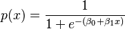
- p(x) is the probability of passing the exam.
- x is the number of hours studied.
- e is a special mathematical number (about 2.718).
- β₀ and β₁ are numbers that the model figures out to make the curve fit the data best. They tell us how much studying affects the chance of passing.
Finding the Best Fit
To find the best β₀ and β₁ values, we use a method called "maximum likelihood estimation." This method tries to find the values that make the observed data (the hours studied and pass/fail results) most likely to happen. It's like finding the curve that passes closest to all the data points.
For our example, the best values found are:
- β₀ is about -4.1
- β₁ is about 1.5
Making Predictions
Once we have these numbers, we can use the formula to predict the chance of passing for any number of study hours.
- Student studies 2 hours:
* The chance of passing is about 0.25 (or 25%).
- Student studies 4 hours:
* The chance of passing is about 0.87 (or 87%).
This table shows the estimated chance of passing for different study hours:
| Hours of study (x) |
Passing exam | ||
|---|---|---|---|
| Log-odds (t) | Odds (et) | Probability (p) | |
| 1 | −2.57 | 0.076 ≈ 1:13.1 | 0.07 |
| 2 | −1.07 | 0.34 ≈ 1:2.91 | 0.26 |
| 2.7 | 0 | 1 | 0.50 |
| 3 | 0.44 | 1.55 | 0.61 |
| 4 | 1.94 | 6.96 | 0.87 |
| 5 | 3.45 | 31.4 | 0.97 |
Evaluating the Model
After fitting the model, we want to know if our predictions are good. The results for our example show:
| Coefficient | Std. Error | z-value | p-value (Wald) | |
|---|---|---|---|---|
| Intercept (β0) | −4.1 | 1.8 | −2.3 | 0.021 |
| Hours (β1) | 1.5 | 0.6 | 2.4 | 0.017 |
The "p-value" for hours (0.017) is very small. This means that the number of hours studied is a very important factor in predicting whether a student passes the exam.
More Complex Models
This simple example used only one factor (hours studied) and two outcomes (pass/fail). Logistic regression can handle many more factors and even more than two outcomes. For example, you could predict if a student will get an A, B, C, D, or F, based on many different study habits.
How Logistic Regression Works
Logistic regression uses a special "S-shaped" curve called the logistic function. This curve takes any number and squishes it into a value between 0 and 1. This is perfect for probabilities!

The formula for the standard logistic function is: 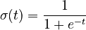
In logistic regression, the t part of this formula is replaced by a simple equation that combines our explanatory variables (like study hours). If we have one variable x, it looks like: 
So, the probability p(x) becomes:
- p(x) is the probability of the "yes" outcome (like passing).
- β₀ is the starting point (like the y-intercept in a line).
- β₁ tells us how much the probability changes for each unit increase in x.
Understanding Odds
Logistic regression also works with "odds." The odds are a way to compare the chance of something happening to the chance of it not happening. For example, if the probability of passing is 0.75, then the probability of failing is 0.25. The odds of passing are 0.75 / 0.25 = 3. This means it's 3 times more likely to pass than to fail.
The logistic model is special because it says that increasing one of the factors (like study hours) changes the odds by a constant amount.

Many Factors, Two Outcomes
We can use many factors (like study hours, attendance, previous grades) to predict a "yes/no" outcome. The formula just gets a bit longer: 
Here, x₁, x₂, etc., are all the different factors we are using. The β values tell us how important each factor is.
Many Factors, Many Outcomes
Logistic regression can also predict outcomes with more than two categories, like predicting if a customer will choose product A, B, or C. This is called multinomial logistic regression. It's a bit more complex, but the idea is the same: use different factors to predict the probability of each possible outcome.
Finding the Best Model
Finding the best β values for a logistic regression model is usually done using computers. The most common method is called Maximum Likelihood Estimation (MLE).
MLE works by trying out different β values until it finds the ones that make the observed data most likely. It's an iterative process, meaning it tries, adjusts, and tries again until it finds the best fit.
Sometimes, the model might not find a perfect fit. This can happen if:
- You have too many factors compared to the number of observations.
- Some factors are too similar to each other (called multicollinearity).
- There are not enough examples for certain outcomes in your data.
Checking How Good the Model Is
After building a logistic regression model, we need to know how well it predicts.
Deviance and Likelihood Ratio Test
In logistic regression, we use something called "deviance" to measure how well the model fits the data. A smaller deviance means a better fit. We compare our model's deviance to a "null model" (a very simple model with no predictors). If our model's deviance is much smaller, it means our factors are really helping to predict the outcome.
For our exam example, the deviance was 11.6661. This number is then checked against a special statistical table (a chi-squared distribution). A very small p-value (like 0.0006) tells us that our model is a much better predictor than just guessing randomly.
Pseudo-R-squared
In other types of regression, people use something called R-squared to show how much of the outcome is explained by the model. Logistic regression doesn't have a direct R-squared, but there are similar measures called "pseudo-R-squared" values that give a general idea of how well the model explains the data.
Checking Individual Factors
We can also check if each individual factor (like "hours studied") is important in the model.
- Likelihood Ratio Test: This is a good way to see if adding a specific factor significantly improves the model's predictions.
- Wald Statistic: This is another test that looks at each factor's importance. However, it can sometimes be less reliable, especially with small amounts of data.
Why Logistic Regression is Different from Linear Regression
Logistic regression is similar to linear regression but has some key differences:
- Outcome: Linear regression predicts a continuous number (like a student's exact score). Logistic regression predicts a "yes/no" outcome or a probability (like the chance of passing).
- Distribution: Linear regression assumes the errors in its predictions follow a normal distribution. Logistic regression assumes the outcomes follow a Bernoulli distribution (which is for "yes/no" events).
- Predictions: Linear regression can predict any number. Logistic regression always predicts a probability between 0 and 1, which makes sense for chances.
Logistic regression is a powerful tool for understanding and predicting events with "yes/no" or categorical outcomes.
History of Logistic Regression
The idea behind the logistic function first appeared in the 1830s and 1840s, developed by Pierre François Verhulst to model how populations grow. He called it "logistic."
Later, in the 1920s, Raymond Pearl and Lowell Reed rediscovered the logistic function for population growth.
In the 1930s, another similar model called the "probit model" became popular, especially in biology.
However, it was Joseph Berkson in the 1940s who really pushed for the logistic model as a general tool, even coining the term "logit." Over time, the logistic model became more popular than the probit model because it was often simpler to use and had useful mathematical properties.
In the 1960s and 1970s, the logistic model was extended to handle more than two outcomes, making it even more useful in many fields.
More Advanced Types of Logistic Regression
There are many advanced versions of logistic regression for different situations:
- Multinomial logistic regression: For when you have more than two unordered outcomes (like predicting which type of animal is in a picture).
- Ordered logistic regression: For when your outcomes have a natural order (like predicting a student's grade: A, B, C, D, F).
- Mixed logit: For more complex situations where choices might be related to each other.
Software for Logistic Regression
Many computer programs and programming languages can perform logistic regression:
These tools make it easy for researchers and data scientists to use logistic regression to make predictions and understand data.
Images for kids
-
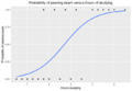
Example graph of a logistic regression curve fitted to data. The curve shows the probability of passing an exam (binary dependent variable) versus hours studying (scalar independent variable).
-

The standard logistic function.
-
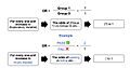
The image represents an outline of what an odds ratio looks like in writing, through a template in addition to the test score example in the "Example" section of the contents. In simple terms, if we hypothetically get an odds ratio of 2 to 1, we can say... "For every one-unit increase in hours studied, the odds of passing (group 1) or failing (group 0) are (expectedly) 2 to 1 (Denis, 2019).
-

This is an example of an SPSS output for a logistic regression model using three explanatory variables (coffee use per week, energy drink use per week, and soda use per week) and two categories (male and female).
-
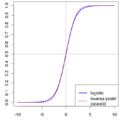
Comparison of logistic function with a scaled inverse probit function (i.e. the CDF of the normal distribution), comparing
 vs.
vs.  , which makes the slopes the same at the origin. This shows the heavier tails of the logistic distribution.

See also
 In Spanish: Regresión logística para niños
