Fermi–Dirac statistics facts for kids

Fermi–Dirac statistics (often called F–D statistics) is a special set of rules in physics. It helps us understand how many tiny, identical particles behave when they are in a system and can't be in the exact same "spot" or energy level at the same time. This rule is called the Pauli exclusion principle.

These rules were created by two scientists, Enrico Fermi and Paul Dirac, who figured them out separately in 1926. F–D statistics is a big part of statistical mechanics, which uses quantum mechanics to study how large groups of particles act.

F–D statistics applies to particles called fermions. Fermions are identical particles that can't be told apart, and they have a special property called "half-integer spin" (like 1/2, 3/2, etc.). When these particles are in a balanced state (called thermodynamic equilibrium), the Pauli exclusion principle means that no two fermions can be in the exact same energy state. This rule has a huge impact on how these systems behave.

A common example of fermions are electrons, which have a spin of 1/2. F–D statistics is often used to describe how electrons act in materials.

There are other types of statistics too:

• Bose–Einstein statistics (B–E statistics) applies to particles called bosons, which have "integer spin" (like 0, 1, 2). Unlike fermions, many bosons *can* be in the same energy state.
• In older, classical physics, Maxwell–Boltzmann statistics (M–B statistics) was used for particles that could be told apart. With M–B statistics, more than one particle could also occupy the same state.

This picture shows how the average number of particles in the lowest energy state changes for the three different types of statistics.

A Look at the Past: How F–D Statistics Helped Physics

Before Fermi–Dirac statistics came along in 1926, scientists had a hard time understanding some things about electrons. For example, when they measured how much heat a metal could hold, it seemed like only a tiny fraction of the electrons were involved in carrying heat, even though many more electrons were part of the electric current. It was also puzzling why the flow of electrons from metals (called "emission currents") didn't change much with temperature.

The problem was that older theories, like the Drude model, treated all electrons as if they were the same and could all contribute to things like heat. This meant that each electron should have added a certain amount to the metal's heat capacity, but experiments showed something different. This mystery remained unsolved until Fermi–Dirac statistics was developed.

Enrico Fermi and Paul Dirac published their work on F–D statistics in 1926. Interestingly, Max Born said that Pascual Jordan had developed similar ideas in 1925, calling it "Pauli statistics," but it wasn't published in time. Dirac himself said that Fermi studied it first, and he called it "Fermi statistics" and the particles "fermions."

F–D statistics quickly became very important. In 1926, Ralph Fowler used it to explain how a star collapses to become a white dwarf. In 1927, Arnold Sommerfeld applied it to electrons in metals, which helped create the free electron model. Then, in 1928, Fowler and Lothar Nordheim used it to explain how electrons are emitted from metals when strong electric fields are applied. Fermi–Dirac statistics is still a key part of physics today.

The Fermi–Dirac Distribution: How Particles Spread Out

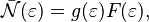
For a system of identical fermions that are in a balanced state (thermodynamic equilibrium), the average number of fermions in a single energy state (let's call it state i) is described by the Fermi–Dirac (F–D) distribution.

In this formula:

• k_B is the Boltzmann constant, a fundamental number in physics.
• T is the absolute temperature of the system.
• ε_i is the energy of that single particle state i.
• μ is the total chemical potential, which is like a measure of how much energy it takes to add a particle to the system.

This distribution is set up so that the total number of particles in all states adds up to the total number of particles in the system.

At a temperature of absolute zero (the coldest possible temperature), μ is equal to the Fermi energy. This is the highest energy an electron can have at absolute zero. For electrons in a semiconductor, μ is often called the Fermi level and is found in the middle of the "energy gap."

The F–D distribution works best when there are many fermions in the system. Since the Pauli exclusion principle says only one fermion can be in each state, the average number of particles in any single state (Failed to parse (Missing <code>texvc</code> executable. Please see math/README to configure.): \bar{n}_i ) will always be between 0 and 1. This also means Failed to parse (Missing <code>texvc</code> executable. Please see math/README to configure.): \bar{n}_i is the probability that a state is occupied.

• Fermi–Dirac distribution
• 

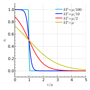
  Energy dependence. This graph shows how the number of particles in a state changes with energy. It's smoother at higher temperatures. When the energy equals the chemical potential (), the average number of particles is 0.5.

• 

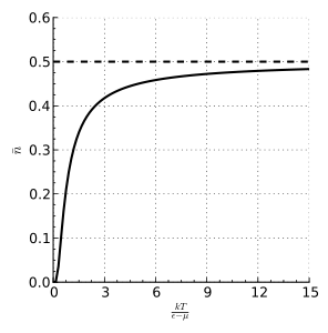
  Temperature dependence for energies higher than the chemical potential. This graph shows how the number of particles in a state changes with temperature.

How Particles Spread Out by Energy

We can also look at how particles are spread out based on their energy. The average number of fermions with a certain energy is found by multiplying the F–D distribution by the `degeneracy` . Degeneracy means the number of different states that all have the same energy .

If is 2 or more, it means there are multiple "spots" with the same energy. So, it's possible for the average number of particles at that energy level, Failed to parse (Missing <code>texvc</code> executable. Please see math/README to configure.): \bar{n}(\varepsilon_i) , to be greater than 1, because different particles can occupy different spots that all have the same energy.

When there's a continuous range of energies, we use something called the `density of states` . This tells us how many states exist per unit of energy. The average number of fermions per unit energy is then:

Here, is called the Fermi function, which is the same as the F–D distribution formula.

This animation shows the Fermi function at different temperatures. The chemical potential (μ) is set at 0.55 eV. Notice how the curve changes as temperature increases.

When Do We Use Fermi-Dirac Statistics?

Fermi–Dirac statistics is essential for understanding systems where particles are very close together or at very low temperatures. In these situations, the quantum rules (like the Pauli exclusion principle) become very important.

However, if particles are far apart or at very high temperatures, the F–D distribution can sometimes be simplified to the Maxwell–Boltzmann statistics. This happens when:

• There are very few particles in each energy state.
• The temperature is so high that particles are spread out over a huge range of energy levels.

The classical rules (Maxwell–Boltzmann) work when the average distance between particles () is much larger than the average de Broglie wavelength () of the particles. The de Broglie wavelength is a quantum property that describes the wave-like nature of particles.

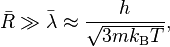
Here, h is the Planck constant and m is the mass of a particle.

Let's look at some examples:

• Electrons in a metal: For electrons in a typical metal at room temperature (around 300 K), the system is far from the classical rules. The electrons are very light and there are many of them, so they are very close together. This means is much smaller than . Therefore, we absolutely need Fermi–Dirac statistics to understand how electrons behave in metals.
• Electrons in a white dwarf star: A white dwarf star is incredibly dense. Even though its surface temperature is very high (around 10,000 K), the electrons are packed so tightly that their small mass and high concentration mean we cannot use classical physics. Fermi–Dirac statistics is necessary to describe the electrons in a white dwarf.

|