Prime-counting function facts for kids

Kids Encyclopedia Facts

The prime-counting function is a special tool in mathematics that helps us count prime numbers. It's like a prime number counter! We write it as $π$ (x). This function tells you how many prime numbers there are that are less than or equal to a certain number x. For example, if x is 10, the prime numbers less than or equal to 10 are 2, 3, 5, 7. So, $π$ (10) would be 4.

It's important to remember that this $π$ (x) has nothing to do with the famous number pi (about 3.14159...). They just happen to use the same symbol!

The values of

π

(n) for the first 60 positive integers. See how the count of primes grows!

How Many Primes Are There?
- The Prime Number Theorem
- Better Estimates for Primes
Counting Primes: A Big Table
How to Calculate π(x)
Other Ways to Count Primes
- Riemann's Prime-Power Counting Function
- Chebyshev's Functions
Formulas for Prime-Counting Functions
Prime Number Rules
The Riemann Hypothesis
See also

How Many Primes Are There?

Mathematicians are very interested in how fast the number of primes grows as x gets bigger. This is a big question in number theory.

The Prime Number Theorem

Around the late 1700s, mathematicians like Carl Friedrich Gauss and Adrien-Marie Legendre guessed that the number of primes up to x could be estimated using a simple formula: x divided by the natural logarithm of x.

This idea became known as the Prime Number Theorem. It says that as x gets really, really big, the actual number of primes, $π$ (x), gets very close to this estimate.

In 1896, two mathematicians, Jacques Hadamard and Charles Jean de la Vallée-Poussin, independently proved this theorem. They used advanced math involving something called the Riemann zeta function. Later, around 1948, Atle Selberg and Paul Erdős found simpler ways to prove it without using those complex tools.

Better Estimates for Primes

For numbers that aren't super huge, another estimate called the logarithmic integral function (written as li(x)) is often even closer to the actual number of primes.

Mathematicians have found even more precise ways to estimate $π$ (x). For example, for numbers x greater than 229, the difference between the actual count of primes and the li(x) estimate is very small.

Interestingly, for many values of x, li(x) is a bit larger than $π$ (x). But it's known that this difference actually switches back and forth an infinite number of times as x gets larger!

Counting Primes: A Big Table

This table shows how the actual number of primes, $π$ (x), compares to two different estimates: x / log x and li(x). You can see that li(x) is generally a much closer guess!

x	$π$ (x)	$π$ (x) − x / log x	li(x) − $π$ (x)	x / $π$ (x)	x / log x % Error
10	4	0	2	2.500	-8.57%
10²	25	3	5	4.000	13.14%
10³	168	23	10	5.952	13.83%
10⁴	1,229	143	17	8.137	11.66%
10⁵	9,592	906	38	10.425	9.45%
10⁶	78,498	6,116	130	12.739	7.79%
10⁷	664,579	44,158	339	15.047	6.64%
10⁸	5,761,455	332,774	754	17.357	5.78%
10⁹	50,847,534	2,592,592	1,701	19.667	5.10%
10¹⁰	455,052,511	20,758,029	3,104	21.975	4.56%
10¹¹	4,118,054,813	169,923,159	11,588	24.283	4.13%
10¹²	37,607,912,018	1,416,705,193	38,263	26.590	3.77%
10¹³	346,065,536,839	11,992,858,452	108,971	28.896	3.47%
10¹⁴	3,204,941,750,802	102,838,308,636	314,890	31.202	3.21%
10¹⁵	29,844,570,422,669	891,604,962,452	1,052,619	33.507	2.99%
10¹⁶	279,238,341,033,925	7,804,289,844,393	3,214,632	35.812	2.79%
10¹⁷	2,623,557,157,654,233	68,883,734,693,928	7,956,589	38.116	2.63%
10¹⁸	24,739,954,287,740,860	612,483,070,893,536	21,949,555	40.420	2.48%
10¹⁹	234,057,667,276,344,607	5,481,624,169,369,961	99,877,775	42.725	2.34%
10²⁰	2,220,819,602,560,918,840	49,347,193,044,659,702	222,744,644	45.028	2.22%
10²¹	21,127,269,486,018,731,928	446,579,871,578,168,707	597,394,254	47.332	2.11%
10²²	201,467,286,689,315,906,290	4,060,704,006,019,620,994	1,932,355,208	49.636	2.02%
10²³	1,925,320,391,606,803,968,923	37,083,513,766,578,631,309	7,250,186,216	51.939	1.93%
10²⁴	18,435,599,767,349,200,867,866	339,996,354,713,708,049,069	17,146,907,278	54.243	1.84%
10²⁵	176,846,309,399,143,769,411,680	3,128,516,637,843,038,351,228	55,160,980,939	56.546	1.77%
10²⁶	1,699,246,750,872,437,141,327,603	28,883,358,936,853,188,823,261	155,891,678,121	58.850	1.70%
10²⁷	16,352,460,426,841,680,446,427,399	267,479,615,610,131,274,163,365	508,666,658,006	61.153	1.64%
10²⁸	157,589,269,275,973,410,412,739,598	2,484,097,167,669,186,251,622,127	1,427,745,660,374	63.456	1.58%
10²⁹	1,520,698,109,714,272,166,094,258,063	23,130,930,737,541,725,917,951,446	4,551,193,622,464	65.759	1.52%

Graph showing how the ratio of

π

(x) to its estimates changes. As x gets bigger, both estimates get closer to the actual count of primes.

The numbers in this table for very large values of x (like 10²⁴ and beyond) were found by super powerful computers and mathematicians like J. Buethe, Jens Franke, A. Jost, T. Kleinjung, D. J. Platt, D. B. Staple, David Baugh, and Kim Walisch.

How to Calculate $π$ (x)

Finding $π$ (x) for small numbers is easy. You can just list the primes and count them.

Using the Sieve of Eratosthenes

One simple way to find all primes up to a certain number x is to use the sieve of Eratosthenes. This method helps you find all prime numbers up to x, and then you just count how many there are.

Legendre's Method

For larger numbers, mathematicians use more clever ways. Adrien-Marie Legendre came up with a method that uses a principle called inclusion–exclusion principle. It's a bit like counting all numbers, then subtracting those divisible by primes, then adding back those divisible by two primes, and so on.

The Meissel–Lehmer Algorithm

For very, very large numbers, even more advanced methods are needed. Ernst Meissel and later Derrick Henry Lehmer developed a complex way to calculate $π$ (x). This method involves breaking down the problem into smaller parts and using special counting functions.

Using his method, Meissel calculated $π$ (x) for numbers up to 100 million (10⁸). Later, Lehmer used an early computer (an IBM 701) to calculate $π$ (10⁹) (1 billion) correctly, and almost got $π$ (10¹⁰) right!

Other Ways to Count Primes

Besides $π$ (x), mathematicians use other functions that are related to prime counting. These functions are often easier to work with in advanced math.

Riemann's Prime-Power Counting Function

This function, often called $\ \Pi_0(x)\$ or Failed to parse (Missing <code>texvc</code> executable. Please see math/README to configure.): \ J_0(x)\ , counts not just primes, but also powers of primes (like 4 which is 2², or 8 which is 2³, or 9 which is 3²). It gives a smaller "jump" for prime powers.

Chebyshev's Functions

The Chebyshev functions are another set of prime-counting functions. They are called Failed to parse (Missing <code>texvc</code> executable. Please see math/README to configure.): \ \theta(x)\ and Failed to parse (Missing <code>texvc</code> executable. Please see math/README to configure.): \ \psi(x)\ . Instead of just counting, these functions add up the natural logarithm of each prime (or prime power). They are very useful in proving theorems about primes.

Formulas for Prime-Counting Functions

Mathematicians have found amazing formulas that can describe these prime-counting functions. These formulas come in two main types:

Arithmetic formulas: These are based on counting properties of numbers.
Analytic formulas: These use tools from calculus and complex analysis.

The analytic formulas were key to proving the Prime Number Theorem. They connect the distribution of primes to the special properties of the Riemann zeta function.

One famous formula for the Chebyshev function Failed to parse (Missing <code>texvc</code> executable. Please see math/README to configure.): \psi_0(x) involves summing over the "zeros" of the Riemann zeta function. These "zeros" are special points where the zeta function equals zero.

There's also a complex formula for $\Pi_0(x)$ that uses the logarithmic integral function and also sums over these zeta function zeros. These formulas show how deeply connected prime numbers are to other areas of mathematics.

Riemann's explicit formula using the first 200 non-trivial zeros of the zeta function. This shows how the sum of many waves can approximate the step-like prime-counting function.

Prime Number Rules

Mathematicians have also found some useful rules, called inequalities, that give us upper and lower limits for $π$ (x). These rules help us know that $π$ (x) will always be between certain values.

For example, for numbers x 17 or larger, we know that: 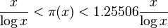$\frac x {\log x} < \pi(x) < 1.25506 \frac x {\log x}$ This means the actual number of primes is always between these two estimates.

There are also inequalities for the nth prime number, written as p_n. These help us estimate the size of the 10th, 100th, or even billionth prime number!

The Riemann Hypothesis

The Riemann hypothesis is one of the biggest unsolved problems in mathematics. If it turns out to be true, it would mean that our estimates for $π$ (x) are even more accurate than we currently know.

It would imply a much tighter boundary on the error in estimating $π$ (x). This would mean that prime numbers are distributed even more regularly and predictably than we currently understand.