Continuous uniform distribution facts for kids

Kids Encyclopedia Facts

Quick facts for kids
**Continuous uniform distribution**
Probability density function Using maximum convention
Cumulative distribution function
Parameters	$- \infty < a < b < \infty$
Support	$[a,b]$
Probability density function (pdf)	$\begin{cases} \frac{1}{b-a} & \text{for } x \in [a,b] \\ 0 & \text{otherwise} \end{cases}$
Cumulative distribution function (cdf)	$\begin{cases} 0 & \text{for } x < a \\ \frac{x-a}{b-a} & \text{for } x \in [a,b] \\ 1 & \text{for } x > b \end{cases}$
Mean	$\tfrac{1}{2}(a+b)$
Median	$\tfrac{1}{2}(a+b)$
Mode	$\text{any value in } (a,b)$
Variance	$\tfrac{1}{12} (b-a)^2$
Skewness	$0$
Excess kurtosis	$- \tfrac{6}{5}$
Entropy	$\ln (b-a)$
Moment-generating function (mgf)	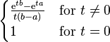$\begin{cases} \frac{ \mathrm{e} ^{tb} - \mathrm{e} ^{ta} }{t(b-a)} & \text{for } t \neq 0 \\ 1 & \text{for } t = 0 \end{cases}$
Characteristic function	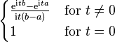$\begin{cases} \frac{ \mathrm{e} ^{ \mathrm{i} tb } - \mathrm{e} ^{ \mathrm{i} ta } }{ \mathrm{i} t(b-a) } & \text{for } t \neq 0 \\ 1 & \text{for } t = 0 \end{cases}$

In probability theory and statistics, the continuous uniform distribution is a type of probability distribution. It's also called a rectangular distribution. Imagine an experiment where any outcome between two specific numbers is equally likely. This is what a uniform distribution describes.

These two numbers are called parameters, usually named a and b. They set the minimum and maximum values for the possible outcomes. For example, if you pick a random number between 0 and 10, any number like 1, 5.5, or 9.9 is equally likely. The distribution is often shortened to Failed to parse (Missing <code>texvc</code> executable. Please see math/README to configure.): U(a,b) , where U stands for uniform.

The length of the interval, which is b minus a, is important. Any section of this interval that has the same length will have the same probability. This distribution is special because it's the "most random" way to spread out possibilities when you only know the lowest and highest possible values.

What is a Uniform Distribution?
Properties of Uniform Distribution
- Moments
- Uniformity
Where is it Used?
History
See also

What is a Uniform Distribution?

Probability Density Function (PDF)

The probability density function (PDF) tells you how likely it is to find a value at a specific point. For a continuous uniform distribution, the PDF is very simple. It's a constant value between a and b, and zero everywhere else.

Think of it like a flat line or a rectangle on a graph. The height of this rectangle is Failed to parse (Missing <code>texvc</code> executable. Please see math/README to configure.): \tfrac{1}{b-a} . This means that every value between a and b has the same "density" or likelihood. If the range (b - a) gets wider, the height of the rectangle gets shorter. This is because the total area under the PDF must always add up to 1.

Cumulative Distribution Function (CDF)

The cumulative distribution function (CDF) tells you the probability that a random value will be less than or equal to a certain number.

For a continuous uniform distribution, the CDF looks like a ramp. It starts at 0 for values below a, goes up in a straight line from a to b, and then stays at 1 for values above b.

Example 1: Finding a Probability

Let's say you have a random variable X that follows a uniform distribution between 0 and 23. This is written as 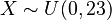Failed to parse (Missing <code>texvc</code> executable. Please see math/README to configure.): X \sim U(0,23) .

What is the probability that X is between 2 and 18? 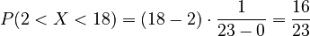Failed to parse (Missing <code>texvc</code> executable. Please see math/README to configure.): P(2 < X < 18) = (18-2) \cdot \frac{1}{23-0} = \frac{16}{23}

This means there's a 16 out of 23 chance that X will fall in that range. On a graph, this probability is the area of a rectangle. The base of the rectangle is 16 (from 18-2), and the height is Failed to parse (Missing <code>texvc</code> executable. Please see math/README to configure.): \tfrac{1}{23} .

Example 2: Conditional Probability

Now, let's try a slightly trickier one. For the same Failed to parse (Missing <code>texvc</code> executable. Please see math/README to configure.): X \sim U(0,23) , what is the probability that X is greater than 12, given that X is already known to be greater than 8?

This is a conditional probability. It changes the "sample space" or the possible range of values. 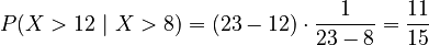Failed to parse (Missing <code>texvc</code> executable. Please see math/README to configure.): P(X > 12 \ | \ X > 8) = (23-12) \cdot \frac{1}{23-8} = \frac{11}{15}

Here, because we know X is greater than 8, our new starting point is 8 instead of 0. The new range is from 8 to 23. The probability is the area of a rectangle with a base of 11 (from 23-12) and a height of Failed to parse (Missing <code>texvc</code> executable. Please see math/README to configure.): \tfrac{1}{15} (from Failed to parse (Missing <code>texvc</code> executable. Please see math/README to configure.): \tfrac{1}{23-8} ).

Standard Uniform Distribution

The standard uniform distribution is a special case. It's a continuous uniform distribution where the minimum value a is 0 and the maximum value b is 1. So, it's Failed to parse (Missing <code>texvc</code> executable. Please see math/README to configure.): U(0,1) .

This standard distribution is very useful. For example, if you have a random number from Failed to parse (Missing <code>texvc</code> executable. Please see math/README to configure.): U(0,1) , you can use it to create random numbers for almost any other type of continuous distribution. This is called the inverse transform sampling method.

Properties of Uniform Distribution

Moments

The mean (average) of a continuous uniform distribution is simply the middle point between a and b. 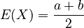Failed to parse (Missing <code>texvc</code> executable. Please see math/README to configure.): E(X) = \frac{a+b}{2}

The variance tells you how spread out the numbers are. For a uniform distribution, it's: 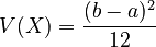Failed to parse (Missing <code>texvc</code> executable. Please see math/README to configure.): V(X) = \frac{(b-a)^2}{12}

Uniformity

One of the most important properties, and why it's called "uniform," is that the probability of a value falling into any section of a fixed length is the same, no matter where that section is located within the distribution's range.

For example, if you have Failed to parse (Missing <code>texvc</code> executable. Please see math/README to configure.): U(0,10) , the chance of a number being between 1 and 2 is the same as the chance of it being between 7 and 8. Both intervals have a length of 1, so their probability is Failed to parse (Missing <code>texvc</code> executable. Please see math/README to configure.): \tfrac{1}{10} .

Where is it Used?

The continuous uniform distribution is easy to work with because its probabilities are simple to calculate. This makes it useful in many real-world situations.

Hypothesis Testing: Scientists use it to test ideas.
Random Sampling: It's used when you need to pick things randomly.
Finance: It can help in financial models.

Often, things that happen naturally, like the emission of radioactive particles, can follow a uniform distribution. The key idea is that every outcome within a certain range is equally likely.

Economics Example

In economics, sometimes things like how long it takes for a product to be delivered (called "lead-time") don't follow a typical pattern. When a brand new product is launched, there might not be any past data to predict its lead-time.

In such cases, the uniform distribution can be very helpful. Even though the exact lead-time is unknown, it's likely to fall between a minimum and maximum value. Using a uniform distribution allows economists to make useful predictions and calculations, even with limited information. It's also chosen because the math is simpler than other distributions.

Generating Random Numbers

Many computer programs have tools to create "pseudo-random numbers." These numbers are designed to act as if they came from a standard uniform distribution (Failed to parse (Missing <code>texvc</code> executable. Please see math/README to configure.): U(0,1) ).

These uniformly distributed numbers are then often used as a starting point to create random numbers that follow other, more complex distributions. For example, the Box–Muller transformation uses two uniform random numbers to create two random numbers that follow a Normal distribution (the famous "bell curve").

Quantization Error

When analog signals (like sound waves) are turned into digital signals (like on a computer), a small error called "quantization error" happens. This error is usually due to rounding. If the original signal is much larger than the smallest digital step, this error often behaves like a uniform distribution. Knowing this helps engineers understand and manage the error.

History

While we don't know exactly when the idea of uniform distribution first came about, it's thought to be linked to the idea of "equiprobability" (meaning "equal probability") in dice games. In the 16th century, Gerolamo Cardano wrote a book called Liber de Ludo Aleae (Book on Games of Chance). It talked about advanced probability calculations for dice, where each side of a die has an equal chance of landing face up. This is a form of uniform distribution, though for discrete (countable) outcomes, not continuous ones.