Computer simulation facts for kids

A 48-hour computer simulation of Typhoon Mawar using the Weather Research and Forecasting model

How a computer model is built, and how experiments, simulations, and theories work together

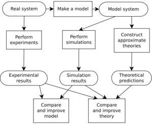
Computer simulation is like creating a digital copy of something real on a computer. This copy helps us guess how the real thing will act or what will happen. Scientists use math to build these digital copies, called mathematical models.

We can check if these models are good by comparing their results to what actually happens in the real world. Computer simulations are super helpful for studying many natural things. This includes physics, astrophysics, climatology (weather), chemistry, biology, and even how things are made. They also help us understand human systems like economics, psychology, and health care.

Running a simulation means using the computer model to see what happens. It helps us learn about new technology. It can also show us how complex systems work when they are too hard to figure out with just math and paper.

Computer simulations use computer programs. Some are small and run fast on tiny devices. Others are huge and can take days to run on many computers linked together. These simulations can study things much bigger than we could ever imagine with old methods. For example, in 1997, a simulation of a desert battle included over 66,000 vehicles! It ran on powerful supercomputers.

Other amazing examples include:

• A model of how materials change, using 1 billion tiny parts.
• A model of the ribosome (a part of living cells) with 2.64 million tiny parts in 2005.
• A full simulation of the life cycle of a tiny living thing called Mycoplasma genitalium in 2012.
• The Blue Brain project, started in 2005. It aims to create the first computer simulation of the entire human brain, down to its smallest parts.

Because simulations need a lot of computer power, scientists use "computer experiments." These help them understand how sure they can be about the results.

What's the Difference: Simulation vs. Model?

Think of it this way:

• A model is like the blueprint or the set of rules (equations) that describe how a system works.
• A computer simulation is the actual process of running that blueprint or rules on a computer. It's like building and testing the thing based on the blueprint.

So, you don't "build a simulation." Instead, you "build a model" (or a simulator). Then you "run the model" or "run a simulation" using that model.

A Brief History of Computer Simulations

Computer simulations grew up with the computer itself. They first became big during World War II. Scientists used them for the Manhattan Project. They modeled how a nuclear explosion would happen. One early simulation used a method called Monte Carlo. It simulated 12 hard balls bouncing around.

Simulations are often used when simple math solutions are not possible. There are many kinds of computer simulations. They all try to show different possible situations for a model. This is useful when it's too hard or impossible to list every single possible state of the model.

How Do Simulations Get Their Data?

Simulations need information to work. How much data they need can be very different. Some might need just a few numbers. For example, simulating electricity on a wire. Others might need huge amounts of data, like weather models.

Where does this information come from?

• It can come from sensors or other real-world devices connected to the model.
• People can enter current or old information by hand.
• Other computer programs or simulations can create the data.

When the data is ready also changes:

• Some data is "fixed" or "invariant." It's built into the simulation's code. This is for things that never change, like the value of pi.
• Data can be loaded when the simulation starts. This might be from files.
• Data can even be given while the simulation is running. This could be from a network of sensors.

Because there are so many ways to get data, special simulation languages have been made. These languages help computers understand the information they receive. It's important for simulations to know how accurate the data is. This helps make sure the results are useful and correct.

Different Kinds of Computer Simulations

Computer models used for simulations can be grouped in different ways:

• Stochastic or Deterministic: Stochastic models use chance or random events. Deterministic models always give the same result if you start with the same information.
• Steady-state or Dynamic: Steady-state models look for a balanced state. Dynamic models show how a system changes over time.
• Continuous or Discrete: Continuous models deal with things that change smoothly, like temperature. Discrete models deal with separate events, like cars passing a point. A special type is discrete event (DES) models.

Here are some specific types:

• A discrete event simulation (DES) keeps track of events in time. It has a list of events sorted by when they should happen. The simulation processes each event, which can trigger new events.
• A continuous dynamic simulation solves math problems that describe how things change over time. It regularly updates the simulation's state. Examples include flight simulators and models of electrical circuits.
• An agent-based simulation models individual things. These could be molecules, cells, or even people. Each "agent" has its own rules and behaviors.
• Distributed models run on many computers connected together, often over the Internet.

Seeing the Results: Visualization

In the past, simulation results were often just tables of numbers. But people found it hard to see patterns quickly this way. Now, computer-generated-imagery (CGI) animation helps a lot!

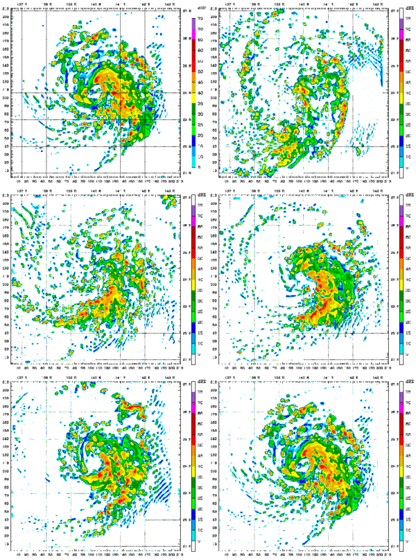
By watching moving images, like a weather map, people can understand trends much faster. They can "see that rain is headed their way" without looking at lots of numbers. These visual displays help us understand complex data.

For example, CGI simulations can show how a tumor might change during medical treatment. It can show time passing as a spinning view of a human head, with the tumor changing inside.

Many other uses of CGI computer simulations are being developed. They help us see huge amounts of data in motion as a simulation runs.

Computer Simulations in Science

Here are some general examples of how computer simulations are used in science:

• Solving complex math problems that describe continuous systems. This includes things like physical cosmology (the universe), fluid dynamics (like climate models), and chemical kinetics.
• Modeling systems where events happen by chance. This is used for things like genetic drift or how small numbers of molecules interact in biochemistry.
• Simulating how tiny materials (nanomaterials) react to forces. This helps understand their properties.

Specific examples in science include:

• Predicting the temperature of water bodies. This uses lots of weather data.
• Agent-based simulation in ecology. It models individual animals, like salmon or trout, when each one behaves differently.
• Models for forecasting river water quality.
• Modeling how the human brain thinks and performs.
• Using molecular modeling for drug discovery.
• Simulating how viruses infect cells.
• Computational fluid dynamics (CFD) simulations. These model how air, water, and other fluids flow. They can be used to design airplane wings or estimate heating needs for buildings.

Some famous computer simulations in science include Donella Meadows' World3 (used in "The Limits to Growth") and James Lovelock's Daisyworld.

Computer Simulations in Everyday Life

Computer simulations are used in many practical ways:

• Studying how air pollutants spread.
• Designing complex things like aircraft and delivery systems.
• Designing noise barriers to reduce roadway noise.
• Training pilots with flight simulators.
• Weather forecasting.
• Predicting risks.
• Simulating electrical circuits.
• Modeling how other computers work (this is called emulation).
• Predicting prices in financial markets.
• Testing how buildings and industrial parts behave under stress.
• Designing industrial processes, like chemical plants.
• Simulating oil reservoirs for petroleum engineering.
• Robot simulators for designing robots.
• Urban simulation models to plan city development.
• Traffic engineering to plan roads and transport systems.
• Modeling car crashes to test safety features in new cars. This saves a lot of money compared to building and crashing real cars. Engineers can see exactly what happens to each part of the car during the crash.
• Modeling crop-soil systems in farming.

For computer simulations to be trusted, the model must be correct. So, checking and proving the model's accuracy is very important. Also, the results should be the same every time you run the simulation with the same starting information. This is especially true for simulations that use random numbers. However, simulations where a human is involved, like flight simulations or computer games, are hard to reproduce exactly because the human's actions change the outcome.

Computer graphics can show the results of a simulation. Animations can help you experience a simulation in real-time, like in training simulations. Animations can also be faster or slower than real-time. For example, fast animations can show how queues build up when people leave a building.

Simulating how a computer program runs can help find more errors than the hardware alone. It can also record useful information for fixing problems, like what instructions were run or how memory changed.

Things to Watch Out For

It's important to check how sensitive the simulation results are. This means understanding how much the results might change if the starting information isn't perfectly accurate. For example, if you're predicting how much oil is in a field, and one key number is only known roughly, then the simulation's final answer might also only be rough, even if it looks very precise.

|

See Also

In Spanish: Simulación (informática) para niños