
Function of a real variable facts for kids
In math, especially when we study shapes and how things change, a function of a real variable is like a rule. It takes a real number as an input. Think of real numbers as all the numbers on a number line, including decimals and fractions. This rule then gives you another number as an output.
Sometimes, a function works for all real numbers. Other times, it only works for a specific group of real numbers. This group is called its domain. For example, a function might only work for positive numbers.
Most of the functions we study are "real functions." This means they take a real number as input and give a real number as output. These functions are super important in engineering, natural sciences, and many other areas. They help us describe how things change and relate to each other.
When a function takes a real number and gives back something else, like a point in space, it can draw a curve. We call these "parametric equations" because they use a variable (like t) to draw the curve.
Contents
What is a Real Function?

A real function is a special kind of function. It takes a real number as input and gives you another real number as output. Imagine you have a machine. You put a number into the machine, and it gives you a new number back. That's what a function does!
The numbers you can put into the machine are called the function's domain. The numbers that come out are its outputs. For real functions, both the inputs and outputs are real numbers. Usually, the domain includes a range of numbers, not just a few separate ones.
Common Examples of Real Functions
Many functions are defined for all real numbers. They are also "continuous," meaning their graph doesn't have any breaks or jumps. They are also "differentiable," which means you can find their slope at any point.
Here are some examples:
- Polynomials: These are functions like f(x) = 2x + 3 or f(x) = x² - 5x + 1. They include simple constant functions (like f(x) = 7) and linear functions (like f(x) = 3x).
- Sine and cosine functions: These are used to describe waves and cycles.
- Exponential functions: These describe things that grow or shrink very quickly, like population growth or radioactive decay.
Some functions are defined everywhere but have jumps.
- The Heaviside step function is an example. It's 0 for negative numbers and 1 for positive numbers, with a jump at zero.
Other functions are defined everywhere and are continuous, but you can't find their slope at every single point.
- The absolute value function (like |x|) is continuous everywhere. But at x = 0, its graph has a sharp corner, so it's not differentiable there.
- The cubic root function (like ³√x) is also continuous everywhere. It's not differentiable at zero because its graph becomes vertical there.
Many common functions are not defined for all real numbers. But where they are defined, they are usually continuous and differentiable.
- A rational function is a fraction where the top and bottom are polynomials (like f(x) = 1/x). It's not defined when the bottom part is zero.
- The tangent function is not defined at certain points, like 90 degrees or 270 degrees, because it involves division by zero at those angles.
- The logarithm function (like log(x)) is only defined for positive numbers. You can't take the logarithm of zero or a negative number.
Some functions are continuous in their whole domain but not differentiable at certain points.
- The square root function (√x) is only defined for numbers zero or greater. It's not differentiable at x = 0 because its graph starts vertically there.
Understanding Functions
A real-valued function of a real variable is a rule that takes a real number (often called x) and gives you another real number (often called f(x)). In this article, we'll just call them "functions" for short.
Some functions work for all real numbers. Others only work for a specific group of numbers. This group is called the function's domain. The domain must always include a range of numbers, not just a few separate ones.
For example, the square root function, f(x) = √x, only works for x values that are zero or positive. So, its domain is all real numbers greater than or equal to zero.
What is the Image of a Function?
The image of a function is the set of all possible output values you can get from the function. For a continuous function that works over a connected range of inputs, the image will also be a connected range of outputs. If the function always gives the same output, it's called a constant function.
The "preimage" of a number y is all the x values that make f(x) equal to y. It's like asking: "What input numbers would give me this output?"
The Domain of a Function
The domain tells you which input numbers a function can use. Sometimes, the domain is clearly stated. If you only use a smaller part of a function's original domain, you create a "restriction" of that function.
On the other hand, sometimes we can make a function's domain bigger. This is often done by "extending by continuity," which means we fill in gaps in the function's graph. Because of this, we don't always need to explicitly state a function's domain.
How Functions Behave: Continuity and Limits

For a long time, mathematicians only studied "continuous functions." A continuous function is one whose graph you can draw without lifting your pencil. It has no sudden jumps or breaks.
To understand continuity, we use the idea of "distance." The distance between two real numbers x and y is simply |x - y|.
A function f is continuous at a point a if, as you get closer and closer to a with your input x, the output f(x) gets closer and closer to f(a). Imagine zooming in on the graph: it looks smooth and connected around that point. A function is continuous if it's continuous at every point in its domain.
The limit of a function describes what value the function is "approaching" as its input gets closer and closer to a certain point. We write this as `L = lim x→a f(x)`. If a function is continuous at a point a, then its limit at a is simply f(a). If a function has a limit at a point on the edge of its domain, we can sometimes "extend" the function to include that point, making it continuous there.
Calculus with Functions
Calculus is a branch of math that studies how things change. It uses functions to do this.
You can combine several functions of a single variable into a "vector." For example, if you have y₁ = f₁(x), y₂ = f₂(x), and so on, you can write them as a vector: `y = (y₁, y₂, ..., yₙ) = [f₁(x), f₂(x), ..., fₙ(x)]`
The "derivative" of this vector is simply the derivatives of each individual function: `dy/dx = (dy₁/dx, dy₂/dx, ..., dyₙ/dx)`
You can also do "line integrals." This is like finding the total effect of a function along a path or curve.
Important Theorems
Calculus has some very important rules and theorems. These include:
- The fundamental theorem of calculus: This theorem connects derivatives and integrals.
- Integration by parts: A technique for solving certain types of integrals.
- Taylor's theorem: This helps us approximate functions with simpler polynomials.
Implicit Functions
Sometimes, a function isn't written in the usual y = f(x) form. Instead, it's given as an equation where x and y are mixed together, like `φ(x,y) = 0`. These are called implicit functions.
For example, the equation for a circle, x² + y² - 1 = 0, is an implicit function. You can't easily write it as y = f(x) because for each x, there are two possible y values (the top half of the circle and the bottom half).
However, if you have a function like y = f(x), you can always rewrite it as an implicit function: `y - f(x) = 0`.
Space Curves in Higher Dimensions

Imagine a point moving through space. Its position can be described by functions of a single variable, usually time t. For example, in 3D space, the position might be given by:
- x = r₁(t)
- y = r₂(t)
- z = r₃(t)
When you put these together, you get a "position vector": `r(t) = [r₁(t), r₂(t), r₃(t)]`
As t changes, this vector draws a one-dimensional path or space curve in 3D space.
Tangent Line to a Curve
If you want to know the direction a moving point is going at a specific moment, you can find the "tangent line" to its path. This line touches the curve at only one point and points in the direction of motion. The slope of this tangent line is related to the derivative of the position functions.
Normal Plane to a Curve
The "normal plane" is a flat surface that is perfectly perpendicular (at a 90-degree angle) to the tangent line at a specific point on the curve.
How it Relates to Motion (Kinematics)

In physics, especially in kinematics (the study of motion), these concepts are very useful.
- The derivative of the position vector, `dr(t)/dt`, tells you the velocity of a particle moving along the path. It's a vector that points along the tangent line.
- The second derivative, `d²r(t)/dt²`, tells you the acceleration of the particle. This vector points towards the center of the curve's bend.
Matrix Functions
A matrix can also be a function of a single variable. This means the numbers inside the matrix change depending on the value of that variable.
For example, a "rotation matrix" in 2D space changes its values based on the angle of rotation. `R(θ) = [[cos θ, -sin θ], [sin θ, cos θ]]` Here, the matrix changes as the angle θ changes.
Another example comes from special relativity. The Lorentz transformation matrix changes based on how fast something is moving.
Complex-Valued Functions of a Real Variable
A complex-valued function of a real variable is similar to a real function, but its output can be a complex number instead of just a real number. A complex number has two parts: a real part and an imaginary part (like 3 + 4i).
If f(x) is a complex-valued function, you can split it into two separate real-valued functions: `f(x) = g(x) + i h(x)` Here, g(x) is the real part, and h(x) is the imaginary part. So, studying complex-valued functions is like studying pairs of real-valued functions.
See also
- Real analysis
- Function of several real variables
- Complex analysis
Images for kids
-
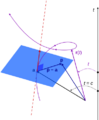
Space curve in 3d. The position vector r is parametrized by a scalar t. At r = a the red line is the tangent to the curve, and the blue plane is normal to the curve.
-
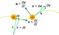
Kinematic quantities of a classical particle: mass m, position r, velocity v, acceleration a.
