AI Mark VIII radar facts for kids

Quick facts for kids
AI Mk. VIII

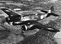
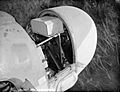
AI Mk. VIIIA in the nose of a Bristol Beaufighter
Country of origin	United Kingdom
Introduced	1941 (1941)
Type	Airborne interception
Frequency	3.3 GHz (S band)
PRF	2500 pps (930 for beacons)
Beamwidth	~12°
Pulsewidth	1 µs (3 µs for beacons)
RPM	1020
Range	400 to 30,000 ft (120–9,140 m)
Altitude	500 ft (150 m) and up
Diameter	28 in (71 cm)
Azimuth	45° to either side
Elevation	45° up and down
Precision	1 to 3° ahead, less to the sides
Power	25 kW
Other Names	ARI 5093, ARI 5049 (Mk. VII)

The AI Mk. VIII (short for Radar, Airborne Interception, Mark VIII) was a very important radar system. It was the first air-to-air radar that used microwave frequencies. This radar was used by Royal Air Force night fighter planes. It helped them find enemy aircraft from late 1941 until the end of World War II. The way it worked, using a moving dish to find and track targets, was used in most aircraft radars until the 1980s.

Work on this radar started in 1939. It got much faster after the cavity magnetron was invented in 1940. This new part worked at a much shorter wavelength (9.1 cm) than older radars (1.5 m). Shorter wavelengths meant smaller antennas could be used. These smaller antennas could aim the radar beam much better. Older radars like the AI Mk. IV couldn't see planes flying low. This was because their wide radar beam bounced off the ground. The Mk. VIII could avoid this by pointing its antenna upwards. This allowed it to see any aircraft at or above the horizon.

The Mk. VIII design was ready in late 1941. This was when the Luftwaffe (German air force) started low-level attacks. An early version, the Mk. VII, was first used on the Bristol Beaufighter in November 1941. A few of these were sent to units in the UK. They helped cover low-flying targets. Planes with Mk. IV radars handled targets at higher altitudes. The improved Mk. VIIIA came out next. The final Mk. VIII arrived in early 1942. It had more power and better electronics. It came just as more De Havilland Mosquito planes were being made. These quickly replaced the Beaufighters in RAF squadrons. Mosquitoes with Mk. VIII radars became the top night fighters from 1943 until the end of the war.

The Mk. VIII led to several other versions. One was the AI Mk. IX, which could "lock on" to targets. This made it easier to catch enemy planes. But problems, including a serious accident, delayed the Mk. IX. It never saw full service. Later in the war, many UK planes used the US SCR-720 radar. This was called AI Mk. X in the RAF. It worked like the Mk. VIII but had a different display. This display offered some advantages. The basic system kept improving. The Mk. IX even reappeared in a very advanced form as the AI.17 in the 1950s.

How Radar Was Developed

Early Radar Ideas

In 1935, the Daventry Experiment showed that radar was possible. This led to the Air Ministry Experimental Station (AMES) being set up. AMES was at Bawdsey Manor to develop radar. Their main goal was to build the Chain Home (CH) system. This system gave early warnings of enemy air raids. As the team grew, they worked on other projects too.

One of these projects came from Henry Tizard in 1938. He worried that Chain Home might not be enough. He thought the Luftwaffe might switch to bombing at night. At night, a fighter pilot could only see a target from about 1,000 yards away. Chain Home couldn't guide pilots that closely. Robert Watson-Watt brought up Tizard's concerns. "Taffy" Bowen offered to work on a new system. This system would fit in planes. It would help pilots find targets at night.

Radio antennas need to be about as long as the radio signal's wavelength. This helps them work well. Chain Home used wavelengths from 10 to 50 meters. This meant antennas had to be at least 5 to 10 meters long. This was too big for an aircraft. Bowen started working on a new system with shorter wavelengths. He first tried 6.7 meters, then settled on 1.5 meters. This was the shortest wavelength possible with the technology at the time. This system became known as Airborne Interception radar (AI). Bowen worked on AI from 1936 to 1940.

During tests of an early 1.5-meter radar, the team couldn't find any aircraft. But they easily picked up large objects like cranes and ships. More tests showed it could find ships at sea. This led to a demonstration where they tracked Royal Navy ships in bad weather. The RAF Coastal Command became very interested. They saw it as a way to find enemy ships and U-boats. The British Army also wanted to use it to aim guns at ships. So, work on AI for aircraft largely stopped for a while.

Developing AI Radar

In 1939, with war coming, the team returned to AI radar. Unlike the successful anti-shipping radars, air-to-air radar had many problems. The main issues were not enough maximum range and too much minimum range. This made it hard to find targets and then see them up close.

Like Chain Home, AI radar sent out a strong pulse in one direction. This lit up the sky in front of the plane. Echoes from aircraft were picked up by several antennas. By comparing signal strength, the target's direction could be found. But the signal also hit the ground and bounced back. This ground reflection was so strong it overwhelmed the receiver. This meant anything beyond about 3 miles was hidden by noise. This left little room to detect targets.

Another problem was not being able to detect targets up close. The radar's transmitter signal was hard to turn off quickly. It was still sending out a small signal when echoes from nearby targets came back. Also, the strong signal could leak into the receiver. This caused it to stop working for a short time. These effects limited the closest detection range to about 800 feet. This was barely close enough for a pilot to see the target at night. Efforts were made to fix this, and Bowen thought they had a solution.

However, the Air Ministry was desperate for AI radar. They made the team build prototype Mk. III units by hand. These were not ready for real use. While these radars were rushed to squadrons, work on fixing the "minimum range" problem stopped. Arthur Tedder later said this was a "fatal mistake."

Early Microwave Work

The Airborne Group started experimenting with microwaves in 1938. They found that certain tubes could work at wavelengths as short as 30 cm. But these tubes had very low power. Also, the receivers weren't very sensitive at these frequencies. This meant detection ranges were very short, almost useless. The group stopped working on it for a while.

But the Admiralty kept pushing for microwaves. The 1.5-meter radars were good for large ships. But they couldn't see smaller objects like U-boat conning towers. This is because objects need to be several times larger than the wavelength to reflect well. The Admiralty controlled tube development in the UK. So, they continued to develop suitable tubes.

Bowen and C. S. Wright from the Admiralty met in 1939. They talked about microwave airborne radar. Bowen agreed that the AI radar's range limits were due to its wide beam. He thought narrowing the beam would fix this. A 10-degree beam would work. An aircraft nose could hold a radar antenna about 30 inches wide. This meant an antenna with poles shorter than 15 cm was needed. If the antenna had to move, 10 cm (around 3 GHz) would be perfect. This matched Wright's needs for a ship radar to find U-boats.

Both groups wanted a 10 cm system. Tizard visited the General Electric Company's (GEC) Hirst Research Centre in November 1939. He discussed the issue. Watt followed up with a visit. This led to a contract on December 29, 1939, for a microwave AI radar. The Birmingham University also got a contract for suitable tubes. Bowen set up a meeting between GEC and EMI in January. This helped them work together on AI.

The Birmingham group was led by Mark Oliphant. They decided to base their work on the klystron concept. Klystrons were invented in 1936 but had low power. Oliphant's team used new tube-making methods. By late 1939, they had a tube that could deliver 400 Watts.

AIS Radar Begins

Watt moved to Air Ministry headquarters. Albert Percival Rowe took over managing the radar teams at Bawdsey. Rowe had problems working with Bowen and others. When the war started, AMES moved to Dundee. The AI team was sent to a small airfield at Perth. Both places were not good for their work.

In February 1940, Rowe started a new AI team. Herbert Skinner led it. Skinner had Bernard Lovell and Alan Lloyd Hodgkin look into antenna designs for microwave radars. On March 5, they visited GEC labs. They saw progress on a radar using VT90 tubes. These tubes now had useful power at 50 cm wavelengths.

Lovell and Hodgkin got a low-power klystron. They started testing horn antennas. These antennas would be much more accurate than the Yagi antennas used on the Mk. IV. Instead of sending radar signals everywhere, this system would act like a flashlight. It would point the radar beam where they wanted. This would also help avoid ground reflections. They could just point the antenna away from the ground. With a 10-degree beam, a horizontal antenna would still send some signal downwards. If the plane flew at 1,000 feet, the beam wouldn't hit the ground until about 995 feet in front. This left room to detect low-flying targets. Lovell built horns with the needed 10-degree accuracy. But they were over a yard long, too big for a fighter plane.

Skinner suggested trying a parabolic dish reflector. This was placed behind a dipole antenna. On June 11, 1940, they found it gave similar accuracy. But it was only 20 cm deep, small enough for a fighter's nose. The next day, Lovell moved the dipole back and forth. He found it moved the beam up to 8 degrees for a 5 cm movement. He felt the "aerial problem was 75 percent solved." Later tests showed the beam could move up to 25 degrees.

After months at Dundee, Rowe agreed the location was bad. He planned to move to Worth Matravers. In May 1940, Skinner moved with scientists from Dundee. Lovell and Hodgkin also moved. They settled in huts at St Alban's Head.

The Cavity Magnetron

While Oliphant's group tried to make their klystrons more powerful, they also looked at other designs. Two researchers, John Randall and Harry Boot, were given a task. They were to adapt a klystron, but it didn't help. They decided to try new ideas.

Most microwave generators worked similarly back then. Electrons moved from a cathode to an anode. Along the way, they passed through hollow copper rings called resonators. As electrons passed, they made the ring vibrate at radio frequencies. This could be used as a signal. The problem was getting enough energy into the resonators. Electrons only gave a small amount of energy each time. To get useful radio energy, electrons had to pass the resonators many times. Or, huge electron currents were needed.

Randall and Boot thought about using many resonators. But this made the tubes too long. Then, one remembered that wire loops with a gap also resonated. This effect was first seen by Heinrich Hertz. Using these loops, a resonator could sit beside the electron stream. If the electron beam moved in a circle, it could pass many loops repeatedly. This would put much more energy into the cavities. And it would still be small.

To make the electrons move in a circle, they used a magnetron. A magnetron uses a magnetic field to control electrons. This was different from using an electrically charged grid. Earlier magnetrons could create small microwaves. But not much work had been done on them.

Randall and Boot combined the magnetron idea with resonator loops. They drilled holes in solid copper. This idea came from W. W. Hansen's work on klystrons. They built a model of what they called the resonant cavity magnetron. They put it in a glass case with a vacuum pump. Then they put the whole thing between the poles of a strong horseshoe magnet. This made the electrons move in a circle.

They tried it for the first time on February 21, 1940. The tube immediately produced 400 Watts of 10 cm (3 GHz) microwaves. Within days, they saw it made fluorescent tubes light up across the room. They quickly figured out it was making about 500 Watts. This was already better than klystrons. They pushed it over 1,000 Watts within weeks. The main Birmingham team stopped working on klystrons. They started on this new cavity magnetron. By summer, they had ones producing 15 kW. In April, GEC was told about their work. They were asked if they could improve the design.

First Magnetron Radar

On May 22, Philip Dee visited the magnetron lab. He was not allowed to tell anyone else in the AIS group about it. He just wrote that he saw the lab's klystron and magnetrons. He didn't say the magnetron was a new design. He did give Lovell a more powerful klystron for antenna tests. This klystron had problems. Its heating parts often burned out. This meant disconnecting it from water, unsealing it, fixing it, and reassembling it. Dee wrote about the messy conditions. Skinner also used the klystron's output to light his cigarettes.

GEC worked on a sealed magnetron. This meant it didn't need an external vacuum pump. They invented a new sealing method using gold wire. They adapted a Colt revolver chamber for drilling. In early July 1940, they made the E1188. It produced 1 kW at 10 cm, like the original. In a few weeks, they improved it. They went from six to eight resonators. They also changed the cathode. The new E1189 could make 10 kW of power at 9.1 cm. This was ten times better than any existing microwave device. The second E1189 was sent to the AMRE lab on July 19.

The first E1189 went to the US in August. It was part of the Tizard Mission. By spring 1940, Bowen was being sidelined in AI radar. This was due to his fights with Rowe. Watt reorganized the AI teams, leaving Bowen out. Bowen joined the Tizard Mission. He secretly carried the E1189. He showed it to the US delegates, who were amazed. They had nothing like it. This caused some confusion. The blueprints they got were for the older six-chamber version.

Lovell continued his antenna design work using klystrons. He finished on July 22. The team then started putting the magnetron radar together. J. R. Atkinson and W. E. Burcham made a pulsed power source. Skinner and A. G. Ward worked on a receiver. At first, they had no way to switch the antenna between sending and receiving. So, they used two antennas side-by-side. One for sending, one for receiving.

On August 8, they were testing this setup. They got a signal from a nearby fishing hut. With the antenna still pointed the same way, they accidentally detected an aircraft. This happened at 6 pm on August 12. The next day, Dee, Watt, and Rowe were there. No aircraft were available. So, the team showed the system by detecting a tin sheet. Reg Batt was bicycling across a nearby cliff with it. This showed the radar could ignore ground reflections. It could detect targets at very low altitudes. Interest in the 1.5-meter systems began to fade.

In July or August, Dee was put in charge of developing a practical 10 cm radar. It was called AIS, for sentimetric. Dee complained that his team and GEC were making similar systems. AIS used a 10 cm magnetron. GEC used Micropup tubes, which now worked at 25 cm. On August 22, 1940, a GEC team visited the AIS lab. The AIS team showed their system. They detected a Fairey Battle light bomber at 2 miles. This was much better than the GEC set. Soon after, Rowe got orders from Watt. All AIS development was put in Dee's hands.

GL Radar Side Project

The AI team moved from St. Alban's to Leeson House. This was a former girls' school. A new lab had to be built there. This caused more delays. But by late summer 1940, the magnetron system was working at the new site.

Meanwhile, the Army was impressed with the 25 cm experimental radars. They wanted to use it as a range finder for Gun Laying radar. Operators would point the radar at targets. Then, the radar info would go to computers that aimed the guns. The 25 cm set's limited power wasn't a big problem. The range would be short, and targets large. The Army's Air Defence Experimental Establishment (ADEE) worked on this. They used the klystron design from Birmingham. British Thomson-Houston (BTH) was their industry partner.

According to Dee, Rowe tried to take over this project in September 1940. After a meeting, Rowe built a GL team. He used several AIS team members. He told them to focus on the GL problem for a month or two. This caused tension between Dee and Rowe. Dee claimed Rowe was "trying to steal the GL problem from the ADEE." He said "only Hodgkin is carrying on undisturbed with AIS."

Lovell said this wasn't as big a problem as Dee thought. The klystron work in Birmingham was partly for Army GL purposes. So, it was fair to use it for that. Lovell's main task was developing conical scanning. This greatly improved radar beam accuracy. It made it accurate enough to aim guns directly. This would be useful for any centimetric radar, including AIS.

On October 21, Edgar Ludlow-Hewitt visited the team. After the visit, Rowe told the team a GL set had to be ready in two weeks. By November 6, Robinson had a prototype. But by November 25, he sent a memo saying it only worked for two days in 19. In December, he was told to take the work to BTH. On December 30, 1940, Dee wrote in his diary: "The GL fiasco has ended up with the whole thing being moved en bloc to BTH."

The project left AMRE's hands. But BTH continued development. The Ministry of Supply changed the plan to use a magnetron in January 1941. This needed more work. But it made a much better radar. The first set was delivered for testing on May 31. Information was then given to Canadian and US companies. Canadian versions became GL Mk. III radar. The US team at the Radiation Laboratory added automatic scanning. This created the excellent SCR-584 radar.

Scanning for Targets

The AIS team went back to airborne interception. They had a complete radar system. But it could only be pointed like a flashlight. This was fine for aiming guns. But for interception, it needed to find targets anywhere in front of the fighter. The team started thinking about how to scan the radar beam.

They first thought about spinning the radar dish horizontally. Then, they would angle it up and down a few degrees with each spin. This "helical-scan" would create a spiral pattern. But it had two problems. The dish spent half its time pointing backward. This limited the energy sent forward. Also, the microwave energy had to go through a rotating connection. At a meeting on October 25, they decided to use the helical-scan. GEC solved the "half-time" problem. They used two dishes back-to-back. They switched the magnetron's output to the dish facing forward. They thought it would be ready by December 1940. But it took much longer.

By chance, in July 1940, Hodgkin met A.W. Whitaker of Nash & Thompson. They talked about the scanning problem. Hodgkin described their idea of moving the dipole at the center of the dish up and down. At the same time, the dish itself moved right and left. Hodgkin wasn't sure this was a good idea. Whitaker built the first version in November. They found the two motions caused huge vibrations. Lovell and Hodgkin thought of a new idea. The parabolic reflector would rotate around the plane's nose. This would trace out circles. By smoothly increasing the reflector's angle, it would create a spiral scan. Whitaker quickly built this system. It scanned a cone-shaped area 45 degrees on either side of the nose.

The spiral and helical scan systems showed data differently. The helical-scan system moved the dish horizontally. It created stripes across the screen. It scanned up and down, making lines above or below the last pass. This was like a television screen. Echoes made the signal brighter, creating a "blip." The blip's location showed the target's direction relative to the plane's nose. The further the blip from the center, the further the target was from the center line. This display didn't directly show range.

The spiral-scan system was a rotating version of a normal A-scope display. In an A-scope, a line moves across the screen. Blips show the range to the target along the line the radar is pointing. For spiral-scan, the line rotated around the display. Blips showed two things: the target's angle from the center line, and its range (distance from the center). What was lost was a direct measure of the angle. A blip in the upper right showed the target was in that direction. But it didn't say if it was five, ten, or twenty degrees off.

Later, they realized the spiral-scan did show angle-off info. The radar beam was about five degrees wide. It would see some return even if the target wasn't centered. A target far from the center would only be seen when the dish pointed right at it. This made a short arc on the display, about 10 degrees long. A target closer to the center would be seen strongly when the dish pointed left. It would still get a small signal when pointed right. This meant it produced a changing return almost through the entire rotation. This created a much longer arc, or a full circle if the target was straight ahead.

More Development

In autumn 1940, AMRE ordered a plane with a nose that radar signals could pass through. Indestructo Glass suggested using 8 mm thick Perspex. The AMRE team preferred a composite material. The Perspex idea was chosen. In December 1940, Bristol Blenheim N3522 arrived. This was a night fighter version of the Blenheim V. It came to RAF Christchurch, the closest airfield. They had trouble mounting the nose to the plane. It wasn't until spring 1941 that Indestructo delivered good radomes.

While this happened, teams kept developing the system. Burcham and Atkinson worked on the transmitter. They tried to make very short power pulses for the magnetron. They used two tubes, a thyratron and a pentode. This made 1 µs pulses at 15 kW. GEC preferred a single thyratron design, but it was dropped. The AMRE design was pushed to 50 kW. This produced 10 kW of microwaves at 2500 pulses per second.

Skinner worked on a crystal detector. This involved endless tests of different crystals. Lovell remembered Skinner "tapping a crystal with his finger until the whisker found the sensitive spot." This led to using a tungsten whisker on silicon glass. It was sealed in a wax-filled glass tube. Oliphant's team in Birmingham continued these tests. They developed a sealed version.

The radio receiver was harder. They decided to use the same basic receiver as the Mk. IV radar. This was a television receiver designed by Pye Ltd. It picked up BBC signals at 45 MHz. It was adapted for the Mk. IV's ~200 MHz. It used an intermediate frequency stage of a superheterodyne system. They added a tube to step down the frequency from 193 MHz to 45 MHz. In theory, this should work for AIS's 3 GHz. But the magnetron's frequency drifted. It changed slightly with each pulse. It changed a lot as it heated and cooled. A fixed-frequency step-down wouldn't work. After trying different designs, they gave up.

Robert W. Sutton from the Admiralty Signals Establishment found a solution. He designed a new tube, now called the Sutton tube. It was a reflex klystron. It took a tiny bit of output from the magnetron. This made electrons passing by it follow the radio signal pattern. Normally, this would go to a second resonator. But in the Sutton tube, electrons hit a high-voltage plate. This reflected them back. By controlling the reflector's voltage, electrons gained or lost speed. This created a different frequency signal as they passed the cavity again. The original and new frequencies combined. This made a new signal for the receiver. Sutton delivered one producing 300 mW in October 1940.

One problem remained: needing two antennas for sending and receiving. Lovell tried using two dipoles in front of one dish. But too much signal leaked through. This burned out the crystal detectors. On December 30, 1940, Dee noted no solution had been found. Crystals still only lasted a few hours. Epsley of GEC suggested another idea. He used spark gap tubes and dummy loads to switch off the receiver. This worked, but ¾ of the signal was lost. Despite this, they decided to use it for the Blenheim in February 1941.

Flight Testing the Radar

In January 1941, scanner units from GEC and Nash & Thompson arrived for testing. The aircraft was still being fitted with the radome (radar cover). So, the team tested both units to see which was better. Watching the spiral scanner work amazed the team. Dee later wrote that RAF staff doubted the scientists' sanity. The system rotated so fast it looked like it wanted to fly out of the plane.

By March 1941, the first AIS unit was ready for flight tests. It was put on Blenheim N3522. Hodgkin and Edwards flew it on March 10. After small fuse problems, they found their target aircraft. It was at 5,000 to 7,000 feet, at about 2,500 feet altitude. The Mk. IV would only have a range of 2,500 feet at this altitude. Using a Battle plane as a target, they soon reached 2 to 3 miles. Tests continued through October. Many high-ranking officials watched.

At first, the closest detection range was over 1,000 feet. The RAF wanted 500 feet. Edwards and Downing worked on this for over six months. They reliably reduced it to 200 to 500 feet. This was a big improvement over AI Mk. IV, which was still around 800 feet. By this time, the Air Ministry ordered the system into production. This was in August 1941, as AIS Mk. I. It was later renamed AI Mk. VII.

The team thought the system would detect targets up to 10 miles away. But it rarely went beyond 3 miles. This was mostly due to the inefficient system used to block the receiver during transmission. This wasted most of the radio energy. Arthur Cooke found the final solution. He suggested using the Sutton tube filled with a dilute gas as a switch. During transmission, the magnetron's power would ionize the gas. This would block the signal from reaching the output. When the pulse ended, the gas would quickly de-ionize. This allowed signals to flow through. Skinner, Ward, and Starr developed this. They tried helium and hydrogen. They settled on a tiny amount of water vapor and argon. This "soft Sutton tube" went into production as the CV43. The first ones arrived in summer 1941.

These tests also showed two useful features of the spiral scan system. First, the scanning pattern crossed the ground when pointed down. This created curved stripes on the lower part of the display. This was like an artificial horizon. Radar operators found it very useful. They could see if the pilot was flying correctly. Everyone was surprised by this, even though it seemed obvious later.

The other surprise was that ground returns caused a false signal. It always appeared at the plane's current altitude. This was like the Mk. IV. But here, the signal was much smaller when the dish wasn't pointed down. Instead of a wall of noise, it made a faint ring. Targets on either side were still visible. The ring was wide at first. After months, Hodgkin and Edwards added a tuning control. This muted weaker signals. It left a sharp ring showing the plane's altitude. This was also useful. Operators could see if they were at the same altitude as their target.

Finally, the team noticed false echoes during heavy rain. They saw the potential for using it as a weather system. But they thought shorter wavelengths would work better. So, they didn't pursue it then.

More Development

Over the summer, the experimental radar was used against submarines. The first test was on April 30, 1941, against HMS Sea Lion. A second was on August 10–12 against ORP Sokół. These showed that AIS could detect submarines with only their conning tower showing. This led to orders for Air-to-Surface Vessel radars based on AIS electronics.

A second Blenheim, V6000, became available. The team used it to test other scanning ideas. They left N3522 with the spiral-scan system. One test was a manual scanning system. The operator would scan the sky using controls. Once a target was found, they could flip a switch. The system would then track it automatically. After much effort, they decided this didn't work. Mechanical scanning systems were better.

The team then compared helical vs. spiral scanners. The GEC helical system was put in V6000. After many tests, they couldn't decide which was better. Work on these systems stopped. The pressure to install the Mk. VII units, which were now being made faster, became urgent. This also seems to be why US versions, called SCR-520, were largely ignored. Bowen noted the confusion during the rush to install.

Mk. VII Enters Service

In spring 1941, the Luftwaffe increased its night bombing, the Blitz. Night fighter groups were getting better. More Beaufighters with Mk. IV were available. The first ground controlled intercept radars also helped. These greatly improved how interceptions were set up. Losses for night fighters grew through the spring. They roughly doubled each month until the Luftwaffe stopped the Blitz in late May.

During this time, the Germans noticed planes dropping mines often returned safely. These planes flew low, usually under 5,000 feet. They started using this to their advantage. They chose targets near the coast and flew low. Their success was because CH radar's lowest detection angle was 1.5 degrees above the horizon. This meant planes could get very close before being detected. This left little time to intercept. Watt quickly responded. He took over deliveries of a British Army radar. It was for detecting ships in the English Channel. He mounted them on tall masts for a long horizon. He renamed them Chain Home Low (CHL). CHL worked down to about 500 feet.

CHL detected raids, but Mk. IV night fighters couldn't stop them. Below 5,000 feet, seeing the target was almost impossible. AIS sets were perfect for this gap. This led to a rush to get them into service. A contract for 100 hand-built prototypes was ordered from GEC in May 1941. They were named AI Mk. VII. In late July, Sholto Douglas ordered four sets to be fitted quickly.

By this point, Dee started putting the system on the Bristol Beaufighter. Hodgkin was in charge of getting Bristol to provide a plane with the radome. But the engineer in charge was unwilling. High-level pressure followed. X7579 was quickly adapted. It arrived at Christchurch in September 1941. The Mk. VII had many large equipment boxes. These were not good for production. Hodgkin was surprised how well the work went. The plane was ready for testing on October 2.

American Competition

Bowen stayed in the US after the Tizard mission. He helped create the MIT Radiation Laboratory. Their progress by November 1940 was "remarkable." Bowen worked with RadLab on Project 1. This was a magnetron-based AI radar like the AIS prototype. Their first system, similar to GEC's helical-scan unit, was ready in February 1941. It was put on a Douglas B-18 Bolo bomber. It first flew on March 10, the same day the first AIS set flew in the UK. During this flight, Bowen estimated the maximum range at 10 miles. On their return, they flew past naval yards. They detected a surfaced submarine at 4 to 5 miles.

Hugh Dowding heard of this performance. He was visiting the US and wanted to see it. On April 29, after detecting a target at 2 to 3 miles, Dowding asked about the minimum range. They showed it was about 500 feet. Dowding was impressed. Before returning to the UK, he met James E. Chaney. He told him about the system and pushed for its immediate development for the RAF.

Western Electric got the contract for five more units, called AI-10. One stayed with Western Electric, one with Bell Telephone. One replaced the original setup in the B-18. One went to the National Research Council (NRC) in Canada. The last went to the UK. The UK copy was supposed to go on a Douglas A-20 Havoc or Boston. But these planes weren't available. Instead, the Canadian NRC provided a Boeing 247 airliner. After a test fit, it was shipped to the UK. It arrived at RAF Ford on August 14 as DZ203. It was widely tested and mostly satisfied everyone.

AI-10 performed similarly to AIS systems of the same time. But Bowen found the RAF wasn't eager to buy it. This was due to several reasons. The AMRE team was busy fitting their own equipment. Also, there was a "not invented here" attitude. But two technical issues were key. The system didn't show range directly. It had to switch to a separate display mode that was almost useless. Also, the set was too big for a Beaufighter. It was designed for larger planes like the Havoc.

The US continued work on AI-10. They put it into production as the SCR-520. The SCR-520-B, used in the P-70, weighed 600 lbs. It was spread over six units. The largest was about a yard on a side. Efforts to make a smaller version led to the SCR-720-A. Then came the final SCR-720. It was similar in performance to the 520 but much smaller, weighing 412 lbs.

Mk. VII Enters Service

As Mk. VIIs arrived in October and November 1941, planes were fitted at Christchurch. Then they went to the Fighter Interception Unit (FIU). The FIU took over from scattered experimental units. It centralized all test flights for Fighter Command. This process eventually reached SD flight. They moved to RAF Ford on November 10. Christchurch then became a satellite field for RAF Hurn.

The new FIU flew X7579 with the prototype AIS on November 30. Tests continued until December 14. During a test flight on December 12, operators found a Junkers Ju 88 bomber. It was on a mine-laying patrol over the Thames Estuary. The crew attacked. They damaged the Ju 88. Oil from its engines sprayed their windscreen. They landed safely. This was the first success for AIS. By May 15, these prototype sets had seven enemy planes destroyed and many damaged.

Mk. VIIs arrived in limited numbers. Even in experimental service, they were excellent. An FIU report said they caused much less trouble than early Mk. IV versions. They pushed for two squadrons to be fully equipped quickly.

FIU had its first success with a production Mk. VII on June 5/6, 1942. A Beaufighter caught a Dornier Do 217 over the Thames Estuary and shot it down. Generally, the Mk. VII came into use as German air activity decreased. But the systems kept scoring victories against low-flying aircraft. Mk. VIIs in the UK and Mediterranean claimed 100 victories. This was one for every set made.

Mk. VIII Radar

By the time experimental Mk. VII units arrived, the final Mk. VIII production version was being planned. A big problem was making the radar much smaller. It almost filled the Beaufighter's rear section. Another goal was to use the new Sutton tubes for switching. This was expected to greatly increase the radar's range. They also wanted to use IFF (Identify Friend or Foe) and radio beacons with AIS. Older transponders worked on the original AI Mk. IV frequencies (around 193 MHz).

The transponder problem had grown before AIS. IFF worked by a small receiver/transmitter. It listened for radar pulses. Then it sent a low-power pulse back on the same frequency, but slightly delayed. This signal returned to the radar plane with the original radar signal. When both were shown, the IFF signal made the blip on the screen stretch out. The 1.5-meter radar system was used for many roles. These included AI, ASV, CHL, and new AMES Type 7 GCI radars. To avoid interference, each worked on slightly different frequencies (180 to 210 MHz). The Navy and Army had their own versions. The IFF Mk. II, for Mk. IV, had to be changed repeatedly for new radar frequencies. None of the many models worked with all of them.

The solution was to pick one frequency for all IFF transponders. This was 180 MHz. The transponder radio was tuned only to this frequency. The radar system also added a separate radio for these pulses, called the interrogator. When the radar operator pressed a button, the interrogator sent pulses. These were timed with the radar unit. The IFF unit in the target plane responded with pulses at the same timing. The interrogator's receiver output mixed with the radar's. This made the blip stretch out. On the spiral scan display, the IFF signal appeared as short lines. These lines went out from the middle of the display, like a "sunrise pattern."

For unknown reasons, the team didn't use the same system for radio beacons. Instead, in July 1941, Hodgkin and Clegg decided to use the radar's own frequency. This would need new ground transponders for AIS night fighters. The radar was adapted. A switch changed the pulse repetition frequency from 2,500 to 930 Hz. This stretched the maximum range to 100 miles. To make up for fewer pulses, the pulse width was made longer. Two pulses were sent back-to-back. So, the total power sent out stayed the same.

Also, the magnetron team in Birmingham made a breakthrough. One problem was that each pulse caused slightly different vibrations in the magnetron's cavities. Sometimes they interfered. With some patterns, like the pi mode, signals added up. The tube was much more efficient. James Sayers found that a metal strap between alternating parts of the magnetron's cavities strongly favored the pi mode. This greatly increased power. GEC started making the new CV64, which could operate at 50 kW. These were called strapped magnetrons.

Finally, UK electronics developed ways to make very short, low-power pulses. These were used to create electronic scales on the displays. These scale lines were drawn using the same signals as the main radar pulses. So, they were always perfectly in sync with the radar. This gave accurate distance measurements without needing to calibrate a mechanical scale. The Mk. VIII system drew circles every 2 miles, up to 8 miles. A new display mode was added for the final stages of interception. It increased the pulse rate and expanded the display to 2 miles. The scale generated circles at 2,000-foot intervals.

Production Plans

AIS and Mk. VII were successful. Plans were made to re-equip all night fighters with Mk. VIII. A three-stage plan was set. First, GEC would build 500 sets of the interim Mk. VIIIA. These would be delivered by late 1942. They could use centimetric beacons but had no IFF. An order for 1,500 sets from a new production line went to EKCO. They would add changes based on Mk. VIIIA use and IFF support. The last version would be Mk. VIIIB. It would have more beacon modes and IFF. These would be added as soon as they were ready. But, as Hodgkin noted, there was rivalry between EKCO and GEC. Each wanted to build AI Mk. VIII their own way. The RAF wanted identical sets.

The first hand-built Mk. VIIIA arrived at Christchurch in March 1942. It seems it wasn't given to the FIU. At this point, centimetric radar development got caught up in new concerns. The Luftwaffe was getting better at signals intelligence and night fighter defenses. In June 1942, the Germans started jamming 1.5-meter radars. This led to calls for the AIS team to help get Mk. VIIIA into service quickly. This again delayed improved versions.

Another Move

In February 1942, German battleships Scharnhorst and Gneisenau escaped from Brest, France. This was the Channel Dash. They were not detected until they were in the English Channel. German ground forces had slowly increased radar jamming. British operators hadn't realized this. After this, Lord Mountbatten and Winston Churchill approved a raid. It was on the German radar station at Bruneval, near Le Havre. The Biting raid captured a German Wurzburg radar system and an operator.

In the following weeks, British authorities worried about German retaliation. Intelligence reported a German paratroop battalion arriving. Rowe was ordered to move the unit quickly. Spencer Freeman of the Emergency Service Organisation found a suitable site. He looked at schools and hospitals. While waiting out an air raid, Freeman remembered Malvern College. It was set aside for the Admiralty. But the invasion threat was no longer immediate.

When the team visited the school in April, they found it empty. This was because students were on Easter holidays. They soon returned. H. Gaunt, the headmaster, was worried by mysterious government inspectors. He contacted the Ministry of Works and Planning. He was told a government department would move in. This forced him to move the students for the second time.

ADRDE, the Army group developing gun laying radars, moved in May. It was renamed the Radar Research and Development Establishment (RRDE). Elements of AMRE joined them. AMRE was renamed the Telecommunications Research Establishment (TRE). After arriving, they planned to install the first six AI sets at RAF Defford. RAF fitters would supervise. Then, planes would fly to two fitting stations. These would serve as patterns for new sets. This system worked very well. At its peak, 80 aircraft were delivered a month.

Window Countermeasure

At the same time, a conflict grew between Fighter Command and Bomber Command. Bomber Command was increasing its attacks. But it was losing many planes to Josef Kammhuber's defenses. They pushed for permission to use chaff, called window in the UK. Tests showed it could blind radar systems. Air Chief Charles Frederick Algenon Porter ordered Bomber Command to use window on April 4, 1942. But he canceled the order on May 5. This was due to pressure from Sholto Douglas. Douglas said Germans would copy window quickly. It was unwise to use it until its effect on UK radars was known.

Under Frederick Lindemann, Derek Jackson did many studies. These were at RAF Coltishall. Starting in September, planes with Mk. IV and Mk. VII were tested against window. There were 30 flights. To everyone's dismay, Jackson found Mk. VII's spiral-scan display was more affected by window than Mk. IV's simpler display. When Douglas learned this, he wrote a memo. He asked that window be held back until new radars were developed.

The Germans had already developed their own chaff, called Düppel. They tested it near Berlin and over the Baltic. But Hermann Göring worried that if they used Düppel over the UK, the RAF would copy it. Bomber Command's fleet was growing fast. The RAF would likely benefit more. Göring had most Düppel paperwork destroyed.

Radar in Action

Mk. VIIIA in Service

The first ten Mk. VIIIA radars from GEC arrived in early December 1942. They were quickly installed. They went to squadrons for low-altitude missions. Planes with Mk. IV radars handled high-altitude targets. The first Mk. VIIIA success was on January 20/21, 1943. An FIU plane caught a Do 217 over the Thames. It shot it down after a tough fight.

During this time, the Luftwaffe strengthened its bomber units in France. They planned raids to get back at the RAF's bombing. New planes like the Do 217 K and M models and Ju 88 A-14 were given to Luftflotte 3. They had about 60 of each by late 1942. Their first raid was on January 17/18, 1943. But they met new GL radars on searchlights. New GCI radars guided night fighters. Five of 118 planes were shot down. Three were helped by searchlights. The existing Beaufighters with AI Mk. IV were good enough against this threat.

But Luftflotte 3 also used Focke-Wulf Fw 190s for bombing. These were used as fighter-bombers, or Jabos, during the day. After some losses, Jabos also flew at night. Even at cruising speed, early Beaufighters couldn't catch them. Raids in April went unchallenged. The biggest threat to attackers was landing accidents. Or getting lost and landing at RAF bases. The Jabo force caused little damage. But the RAF quickly brought in new planes like the Beaufighter VI. They equipped them with new radars. However, these planes weren't much faster than the FWs. They weren't good enough.

A better solution to the Jabo problem was arriving. In July 1942, Mosquito Mk. II DD715 was changed for night fighter use. It got a new "thimble" nose and Mk. VIIIA radar. This meant removing the four Browning machine guns. Only the Hispano 20mm cannons in the belly remained. After trials, 97 more Mk. IIs were converted starting in September 1942. A special night-fighter Mosquito, the NF.XII, arrived in February 1943. When German fighters returned on May 16/17, No. 85 Squadron intercepted them. They shot down five Jabos. Operations against Jabos were successful. The Jabo campaign slowed down.

Mk. VIII in Service

The first pre-production Mk. VIII arrived on December 21, 1942. It was fitted to a Beaufighter. This showed that some changes were needed. Even with a magnetron ten times more powerful, normal detection ranges were short. They were about 4 miles. Modified versions started arriving in May. As production increased, these radars went mostly to Mosquitoes. Their numbers grew a lot in late summer. By this time, Jabo raids on large targets had slowed. The Luftwaffe started its biggest mine-laying campaign. In September and October, 37 Luftwaffe planes were destroyed on mine-laying missions.

This part of the war saw Bomber Command's raids on Germany grow. The Luftwaffe tried to defend against these attacks. Luftwaffe raids on the UK dropped a lot, except for mining. This gave RAF night fighter groups time to rest and re-equip. They replaced older Beaufighters and Mosquitoes with new ones. Most were the new Mosquito NF.XII with Mk. VIII. This left the question of what to do with Mk. IV planes. Many found new life as intruders. They used the new Serrate radar detectors.

Operation Steinbock

The Luftwaffe tried one last big bombing campaign against the UK in early 1944. This was Operation Steinbock. Luftflotte 3 gathered 474 bombers. These included newer Junkers Ju 188s and Heinkel He 177s. They also had more Messerschmitt Me 410 heavy fighters as jabos. They would use Düppel, their version of window, for the first time. Some planes had the Truhe navigation system, a copy of the UK Gee. They also had their own Y-Gerät, though it could be jammed.

By this time, the RAF had reorganized for Operation Overlord. Many fighter planes moved to the 2nd Tactical Air Force. Planes for defense were put into the re-created Air Defence of Great Britain (ADGB). ADGB mostly had Mosquito NF.XII, XIII, and XVII. These had Mk. VIII and some Mk. X radars. But many were on other duties. Some units were refitting. Only about 65 night fighters were available.

The first Steinbock raid was planned for December. But problems delayed it until January 21/22, 1944. The Luftwaffe pathfinders used every trick. They dropped white marker flares and marked London in green. Attackers dropped lots of Düppel. This successfully jammed the 1.5-meter radars. Newer centimetric radars had been deployed. These could still guide fighters. Mosquitos of ADGB claimed 16 bombers destroyed or probable. New centimetric guided anti-aircraft artillery added 9 more. Another 18 German planes never returned. They got lost or crashed landing. This was about 10% of the 447 bombers. This loss rate was higher than the Luftwaffe usually caused the RAF. Such losses would quickly deplete their force. For all this effort, bombers dropped only 30 tons on the city. This caused 14 killed and 74 injured. This was a tiny fraction of the Blitz's nightly load. Hitler was furious.

The US opening of Battle of Anzio the next day took 100 bombers from Luftflotte 3. They were sent to Italy. Steinbock attacks continued through February with bad results. By month's end, Mosquitoes claimed 28 planes. Large attacks continued through March. On March 19/20, Joe Singleton and Geoff Haslam of No. 25 Sqn shot down three Ju 88s in 13 minutes. Such events were common. Many crews had multi-kill missions. Smaller raids continued through April. Some harassment raids happened in May. By then, Luftflotte 3's force fell from 695 to 133 planes. RAF losses were about two dozen. Only one was from enemy action.

Fighting the V-1 Flying Bomb

The V-1 flying bomb was first launched at London on June 13. It quickly became a bigger threat than bombers. A defense system was set up on June 15. But the overlapping areas of anti-aircraft guns and fighters caused confusion. After talking to Frederick Alfred Pile, General of the Army's AA units, Air Marshal Roderic Hill reorganized the AA guns. They formed a thin belt along the coast. Fighters operated inland. This greatly improved operations for both forces.

V-1s were launched day and night. They flew at about 350 mph. This was the top speed for many defensive fighters. Mosquito pilots soon learned a trick. They flew over the Channel looking for the V-1 engine flames. When they saw one heading their way, they flew above and to one side. Then they dove on it from the side. This kept the flames in sight. This diving approach let them catch the missile. The problem was knowing when to fire. It was hard to tell range at night with only flames visible. The radar operator called out the range. The pilot fired when they reached 900 to 1,000 feet. The whole thing was dangerous. Radar operator Jimmy Rawnsley remembered one flight:

I looked up as the guns crashed briefly; and I immediately ducked down again. The bomb had burst just 300 yards ahead of us, and we were rushing at over 150 yards a second straight at the heart of the explosion. For a few seconds the jet of air from the ventilator close to my head blew hot and acrid; but we were still flying. Sitting up and looking back, I saw that the air behind us was full of glowing red fragments still fanning out and floating downward.

In total, 8,081 V-1s were fired at the UK from June 13 to September 1. Of these, 1,902 were destroyed by fighters. Another 1,564 were destroyed by anti-aircraft fire. This left 2,340 to reach London.

After this, launching sites were captured. V-1 operations moved to airborne launches from He 111 bombers. In July and August, KG 3 launched almost 400 V-1s. They started during the day but quickly switched to night. KG 3's third group was renamed I.Gruppe/KG 53 in September. They continued the campaign. They kept pulling back towards Germany as Allies advanced. Firings ended on January 14, 1945. By then, 1,012 missiles were fired. 77 He 111s were lost, and 404 missiles were destroyed in flight.

Future Radar Ideas

Lock-Follow System

The idea of "lock-follow" was first written down by Bernard Lovell on March 8, 1941. This system would allow the radar to track targets automatically. Radars with lock-follow were called AIF or AISF.

Lovell had built a ground system for the Navy to detect ships. He adapted it for automatic aircraft tracking. Engineers from several companies joined him. "Freddie" Williams helped create the Velodyne system. It tracked smoothly even with fast-moving targets. This system also sent range info directly to the gyro gunsight. This set it up to fire as soon as the target was seen.

The system used two dipole antennas instead of one. They were slightly offset on either side of the dish's center. This made their beams angle away from each other. Normally, signals from both were added and displayed. This looked like the single-dipole case. The dipole shaft spun rapidly at 800 rpm. A switch was triggered when the dipoles were vertical or horizontal. This activated a circuit that subtracted the signals. The result was the difference in signal strength. This showed which dipole received more energy. This signal then drove the scanner motors. It moved the radar in the right direction.

Interceptions started like normal AIS. The operator searched for targets. When a target was chosen, the operator adjusted a "strobe." This was a time-base circuit that made a ring on the display. When the strobe was over a target's return, a button was pushed. This filtered out signals before or after that range. Only the chosen target remained visible. The tracking circuits then kept the radar dish pointed at the target.

The system worked by autumn 1941. It used Mk. VII electronics and a new 50 kW magnetron. This created the AI Mk. IX. It detected targets at 10 miles. It could lock on at 5 miles. It tracked movements up to 10 degrees per second. Despite this, Lovell was sent to work on the H2S system on January 1, 1942. The Mk. IX was then led by Arthur Ernest Downing. The team still thought it would be ready in 1942.

Mk. IX Radar

In November 1942, the Air Interception Committee discussed the future of AI radar. They wanted several new features. The main idea was an all-around view, like ground-controlled intercept radars. This would let fighters plan their own interceptions. Range was to be extended to at least 10 miles. Minimum range was to be 200 feet. This short minimum range, with half-degree accuracy straight ahead, allowed firing without seeing the target. Other features like lock-follow and accurate range finding were also considered.

Three designs were studied. One was an X band version of the Mk. VIII. It would work at 3 cm instead of 10 cm. The second was a Mk. VIII using spiral-scan instead of helical. The third was Lovell's AIF system. After discussion, the X band idea was dropped. RAF pilots were used to S band equipment. And existing beacons could be used. These outweighed any technical benefits.

When the debate about window started in spring 1942, Downing suggested AIF might be immune. Window (aluminum foil) stops in the air and falls slowly. An AIF locked onto a bomber would see these signals quickly leave the gated range. They would disappear. To test this, a Beaufighter with the AIF prototype flew to Coltishall. Jackson did 13 flights in November to test it against window. These tests showed, to great concern, that the system would lock onto the window instead. It would lose the bomber.

Downing suggested changes to keep a lock with window present. He made these changes over weeks. On December 23, 1942, Downing personally operated the upgraded Mk. IX in a Beaufighter. A second Beaufighter with Jackson dropped window. Jackson heard radio messages about Spitfires investigating "bogies." He worried they meant their planes. Soon after, two Spitfires appeared and fired on both Beaufighters. Jackson's damaged plane made it back. But Downing's plane crashed into the sea, killing everyone.

Mk. X Radar

The loss of the only Mk. IX prototype and its main developer greatly delayed the program. Around the same time, TRE received an SCR-720 unit from the US. This was a smaller, lighter version of the SCR-520. It was suitable for the Beaufighter and Mosquito. The first one arrived in December 1942. Jackson tested it against window in January 1943. Jackson found that by switching the range control, he could set the radar to look at the bomber. The window would quickly go out of range and disappear.

TRE made minor suggestions and upgrades. They ordered 2,900 SCR-720B's, calling them AI Mk. X. However, Western Electric had focused on the SCR-520. This was for the Northrop P-61 Black Widow. This was a large, 15-ton, 66-foot wingspan night fighter. By this time, the P-61 was very delayed. The USAAF started using Beaufighters and Mosquitoes. This led to demands from both USAAF and RAF for SCR-720 production to speed up. Western Electric said initial units would be ready in May 1943. Production quantities would be ready in August.

With the decision made, the Air Ministry finally allowed window to be used in July 1943. It was first used on a raid on Hamburg on July 24/25, 1943. The effects were amazing. German defenses relied on radar. Window created so many false targets that operators didn't know what to do. AA guns fired randomly. Night fighters flew in circles. The attacking force lost only 12 planes. This was 1.5% of the force, about what would happen by chance.

The first SCR-720 was delivered on July 12. It was fitted to Mosquito HK195. It went to the FUI on August 11. It first flew two days later. Small batches were completed on various Mosquito models. Then, production focused on the NF.XIX. This model had Rolls-Royce Merlin 25 engines and stronger wings for external fuel tanks. Unfortunately, Mk. X deliveries were greatly delayed. The first 40 arrived in late autumn. They lacked many requested upgrades. Once adapted, they interfered with aircraft radios. It wasn't until January 1944 that the first Mk. X sets went to squadrons.

More Mk. IX Development

With the Mk. X chosen, the Mk. IX program became less important. New ideas were considered. They thought about adapting the Mk. IX to work in the S-band at 3 cm wavelengths. This would give even higher accuracy from the same antennas. Or similar accuracy from smaller ones. EKCO started adapting Mk. VIII equipment to work at either 9 or 3 cm. But 3 cm magnetrons only made 50 watts of power then. This option was never used.

In a September 23, 1943 memo, Air Commander W. C. Cooper outlined four possible developments:

• AI Mk. IX – the version being developed, with a pilot's display screen.
• AI Mk. IXB – IX with the pilot's display projected on the windscreen.
• AI Mk. IXC – IXB with the pilot's display combined with a gyro gunsight.
• AI Mk. IXD – IXC with a computer to calculate where to aim.

Burcham developed the Mk. IX line in 1943, following the IXB idea. This was later paired with a new 200 kW magnetron. An early version without the pilot's display was tested by the FIU in Mosquito HK946 in December 1943. It returned with many suggestions for upgrades.

Windscreen projection was tried with AI Mk. IV as the Mk. V. But problems were found, and it wasn't used. Several updated versions were tested. By 1943, Mk. V radar was old. The Pilot's Indicator Display (PID) was adapted to the Mk. VIII instead. This system's output was projected into the existing GGS Mk. II gyro gunsight. It was fitted to Mosquito HK419 in late 1943. It went to the FIU for testing in January 1944. It received wide praise.

With Mk. X being installed, all PID work moved to the Mk. IX. The first Mk. IXB with PID was fitted to Mosquito HK311 in 1944. It went to the new Central Fighter Establishment (CFE, formerly FIU) on December 22, 1944. This set also had upgrades from earlier Mk. IX tests. An upgraded HK946 joined it. It was tested a lot from December 1944 to April 1945. The FIU found the lock-follow system didn't work at low altitudes. This was about 2,000 feet over water or 5,000 feet over land. But above these, Mk. IX was better than Mk. X. They said it needed more training than Mk. X. And the display had to be changed so PID didn't block cockpit instruments. The plane returned to Defford with many suggested improvements.

After the War

After the war ended, Mk. IX development stopped. People thought another war was at least a decade away.

In 1947, the Soviet Union introduced its Tupolev Tu-4 bomber. It could reach the UK from bases in Russia. In 1949, the Soviets tested their first atomic bomb. This led to efforts to improve UK radar systems under the ROTOR program. They also wanted a new night fighter that could fight the Tu-4's 350 mph speed. Some work had started on a jet night fighter. But much time and money could be saved by upgrading the Mosquito.

In February 1948, the CFE evaluated the new Mosquito NF.38 with Mk. IXB. They found the low-altitude lock-follow problems remained. This made the Mk. X easier to use. They also noted Mk. IX still had trouble locking on with window. And the PID was too dim for day, too bright at night. They concluded:

The opinion of this Establishment is that AI Mk.9B is operationally unacceptable in freelancing, broadcast control, or bomber support operations. It is, therefore, recommended that AI Mk.9B should not be accepted for service use.

The CFE also rejected the NF.38. Its performance was only slightly better than the late-war NF.36. It was barely better than the B-29/Tu-4. As a night fighter against the Tu-4, it would be useless. Mk. IX was officially canceled in 1949. One Gloster Meteor, VW413, was being converted for Mk. IX tests. Its construction continued for testing in July 1950.

Naval Use

Years later, Lovell learned that a version of the Mk. IX was tested on Motor Gun Boats in 1942. It successfully tracked other boats. It allowed blind-fire of a 2-pounder gun with good accuracy.

How the Mk. VIII Radar Worked

The earlier Mk. VII radars were similar to Mk. VIII. But they used a less powerful CV38 magnetron. This gave about 5 kW of power instead of 25 kW in the Mk. VIII's CV64. This reduced the normal range to about 3 miles. Other performance was the same. Mk. VII lacked inputs for IFF, beacons, or AIBA. The rest of this description is for the Mk. VIII.

Equipment Setup

The Mk. VIII system had two main parts. The transmitter and antenna were in the plane's nose. Most of the receiver and display were inside the cabin.

The nose equipment included the magnetron transmitter and the soft Sutton tube switch. These were in one box on the mounting frame. On the Mosquito, it was near the top. On the Beaufighter, it was at the bottom. This made them easy to reach. The scanner system was in the center of the frame. It rotated the 28 cm parabolic dish 17 times a second. The signal was sent from a small vertical dipole antenna. This was at the end of a post through a hole in the dish. A coaxial cable carried the signal from the magnetron. The parts on the frame included the Type 53 Modulator. It provided 35 Amps and 10 kV pulses. The Type TR.3151 transmitter had the CV64 magnetron, CV43 soft Sutton switch, and a crystal mixer. The Type 50 receiver had its CV67 Sutton tube local oscillator. This stepped down the frequency.

The receiver, time base, and display were inside the cabin. There was plenty of room in the Beaufighter. The radar operator sat at the back. In the Mosquito, the operator sat to the right and slightly behind the pilot. The main entry door was on the left. With the radar installed, there was almost no room to reach the door. So, the time base circuitry was on rails. It could slide up and forward, out of the way. Parts inside included the Type 73 display and the TR.3152 Lucero.

The system got power from the Type 225 power supply. It ran off a power take off shaft on one engine. This made 1,200 W of 80 V AC power. It converted 500 W to DC for instruments that needed it. The scanner motor was hydraulic. It was powered by a pump on one engine. The whole system, including power supply, weighed 212 kg.

Performance of the Radar

The Mk. VIII showed good returns on bomber-sized targets at about 5.5 miles. It could sometimes get returns as far as 6.5 miles in good conditions. The closest detection range was about 400 to 500 feet. This was limited by the pulse width and how long the transmitter signal took to "die down." At short range, the target's arc could merge with the "zero ring." In these cases, a bias control could be adjusted. This silenced the receiver for longer. It suppressed the zero ring, making nearby targets easier to see.

The radar beam was very sharp. The edges of the arc were strong. The target would appear and disappear with little change in brightness. This meant the arcs were sharp. Even small angles would make signals disappear and create a gap. With targets near the center, this was easy to see. The ring would get a gap. This allowed measurements as accurate as one degree. But targets further from the center showed shorter arcs. This made it harder to see small changes in their length.

IFF Use

Mk. VIII was made to work with IFF Mk. III. This system listened for pulses between 160 MHz and 190 MHz. It responded with longer pulses on a slightly different frequency. The magnetron worked at 3.3 GHz. So, it wouldn't trigger the IFF. A second pulsed transmitter was used in the fighters for this. It was called the interrogator (or interrogator/responder), code-named Lucero.

Lucero was connected to the Mk. VIII transmitter. It sent its own 5 µs signal every fifth radar transmission. The IFF Mk. III in the other plane had a receiver. This fed into a transmitter. It amplified and stretched out any received signal. This signal was received by Lucero's responder. It mixed it with the Mk. VIII's own receiver signal. Lucero's antenna sent signals in all directions. So, returns were continuous around the display. They were not related to the main dish's position. This resulted in short line segments. They were spaced every 10 degrees around the display.

Lucero's transmission was faster than the radar's magnetron. This let it send its signal and start receiving the reply. This happened while the main radar pulse was traveling. So, the line segments started closer than the plane sending the response. They ended after it. The radar operator could tell which plane was sending IFF responses. They looked for blips roughly centered along the line segments.

Beacons

Mk. VIII also used radio beacons. These were for long-range guidance to ground-based transponders. Here, the system used transponders on the same frequency as the radar. This was unlike Lucero, which had its own frequencies. The dish had to point downwards to see the ground transponder. So, the transponder sent its response on a slightly different frequency. This helped tell it apart from ground reflections.

The beacon's altitude was known (on the ground). So, the angle display wasn't needed. A switch was flipped by a small cam on the scanner. This happened when it passed the 12 and 6 o'clock positions. It inverted the receiver output. Angular scanning was turned off. The time base moved to the bottom of the screen. Received signals made the time base move left or right. This depended on where the dish was pointed.

Switching to beacon mode slowed the pulse rate. This gave signals more time to travel. It stretched the range to 100 miles. Pulses were also made longer. This kept the total power sent out the same. This switch also made the strobe produce markers every 10 miles instead of 2.

The system normally switched the receiver to the beacon frequency. But the operator could also switch it to the normal transmitter frequency. Then, ground returns would appear. Water and land produced different returns. So, this mode was sometimes useful for finding coastlines, large objects, and ships. It could do this at ranges up to 40 to 50 miles.

AIBA Landing System

The UK used a blind landing system called Standard Beam Approach. It was based on a German system called a Lorenz beam. Lorenz, and Standard, used two radio transmissions. These were picked up by voice radios. Signals came from two antennas at the end of the runway. They switched between the two. They spent 0.2 seconds on the left antenna and 1 second on the right.

To use Lorenz, the radio operator tuned to the airfield's frequency. They listened for "dots" or "dashes." Dots (short 0.2 s pulse) meant they were too far left. They turned right to reach the center. Dashes meant they should turn left. In the center, the receiver heard both signals. They merged to form a steady tone, the equisignal.

During Mk. IV development, new Standard Beam Approach radios were made. They worked on the 1.5-meter band. These were called Beam Approach Beacon System, or BABS. This was also the band for IFF Mk. II. It was similar to the new IFF Mk. III bands. For the Mk. VIII radar, they decided not to make a new microwave transponder. They simply adapted the Lucero system to receive BABS signals. This was called AI Beam Approach system, or AIBA.

For AIBA, the Lucero system sent pulses on 183 MHz. BABS responded with 8 µs pulses on 190.5 MHz. These went to another display mode. It had a single vertical time base 8 miles long. The strobe made markers every 2 miles along it. No switching was used. The signal always made the beam deflect to the right. This created a wide bar. Depending on which side of the runway the plane was on, the operator saw long bars for 0.2 seconds and short ones for 1, or vice versa. If the dot signal was longer, it meant the plane was too far left. Using these signals, the plane could get on the center line. Then, both dot and dash signals were the same length, and the bar stayed steady.

Images for kids

• 

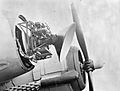
  AI Mk. VIIIA in the nose of a Bristol Beaufighter

• 

  Avro Anson K8758 was used to test radar systems. Its detection of Royal Navy ships in bad weather was the harbinger of the destruction of the German U-boat force.

• 

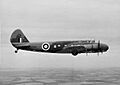
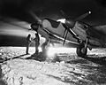
  The Bristol Beaufighter equipped with Mk. IV radar was the world's first truly effective night fighter. "Paddy" Green shot down seven Axis aircraft over three nights in this example.

• 

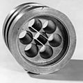
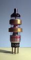
  This original magnetron, about 10 cm across, revolutionised radar development.

• 

  This marker was placed at the former location of AMRE's buildings at St. Alban's Head.

• 

  Leeson House was a significant improvement from the huts they formerly occupied, but the AI team was only here for eighteen months before moving once again.

• 

  The Sutton tube ultimately solved two thorny problems for the AIS team, acting as both a local oscillator as well as a high-speed switch.

• 

  The successful detection of HMS Sea Lion by AIS spelt doom for the German U-boat fleet. By 1943, Coastal Command aircraft with centimetric ASV radars could hunt down submarines with even small portions above water.

• 

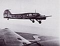
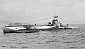
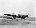
  A formerly Canadian Boeing 247D, DZ203, was used extensively during the war to test US radar systems in the UK.

• 

  Beaufighter X7579 achieved the first success for the microwave radar system.

• 

  Malvern was even more imposing than Bawdsey, and was at last a suitable inland location.

• 

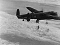
  Bundles of window are dropped from an Avro Lancaster during a raid on Duisburg.

• 

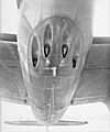
  Installation in the De Havilland Mosquito, like this NF.XIII HK382 of No. 29 Sqn, used a thimble radome that required the removal of the four machine guns formerly in this location.

• 

  The distinctive thimble radome is particularly well displayed in this image of a Mosquito NF.XII in the snow at B51/Lille-Vendeville, France.

• 

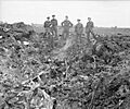
  This crater and debris are all that remains of a Ju 188E-1 shot down by a Mk. VIII-equipped Mosquito NF.XII of 488 Sqn RNZAF on the night of 21 March 1944, near the height of the Steinbock raids.

• 

  This Mosquito NF.XVII of 85 Sqn was covered by the burning oil and debris of a Junkers Ju 188 they shot down on the night of 23/24 March.

• 

  Shooting down a V-1 was dangerous, as this Mosquito FB.VI of 418 Sqn RCAF demonstrates with its burned-off outer fabric.

• 

  The SCR-720, known as AI Mk. X in RAF service, was a relatively compact system, especially compared to the earlier SCR-520.

• 

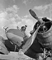
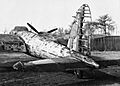
  The Mk. VIIIB as mounted to a framework on the nose of the Mosquito. The electronics were contained in the white box, easily accessible under a removable fuselage panel. The radar dish scanner is mounted on the X-shaped frame.

• 

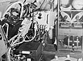
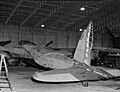
  The Mk. VIIIA display was a complex but compact system, shown here installed on the starboard side of a Beaufighter.

• 

  The IFF/Lucero antenna can be seen projecting downward just behind the guns in this image of the lower fuselage of a Mosquito NF.XIII.